
Science Extension Journal

Science Volume 4 Number 1 September 2022 Scientific Research
School
An Anglican community inspiring
To be a leader in Christian education that is characterised by a global vision that inspires hope
Mission
every learner every experience every day Vision
Values Commitment Compassion Courage Integrity RespectHonor Non Honores
We acknowledge the Dharug, Darkinjung, Wonnarua and Yolŋu peoples who are the traditional custodians of the land on which Barker College, Darkinjung Barker, Ngarralingayil Barker and Dhupuma Barker stand. We pay respect to the Elders past, present and emerging of the Dharug, Darkinjung, Wonnarua and Yolŋu nations and extend that respect to other Indigenous people within the Barker College community.
Senior Editor
Dr Matthew Hill
Creative Direction
Mrs Susan Layton
Dr Matthew Hill
Research Supervisors
Dr Alison Gates
Dr Terena Holdaway-Clarke
Dr Matthew Hill
About the Scientific Research in School Journal

When the New South Wales Education Standards Authority announced a new course “Science Extension” to commence in 2019 we were thrilled that there was an opportunity for a formally-assessed capstone experience in Science for our students. From the perspective of the Barker Institute it was an exciting chance to support students doing academic research, alongside other subjects such as History Extension, Music Extension and English Extension 2.


Where many capstone project courses fail is the at final step of the research process – dissemination. Research is not merely the process of conducing an investigation and writing a report, but sharing it with the wider community so that people can learn, critique, have other student researchers at multiple schools build on the projects published. I am so glad to be able to publish this journal each year now celebrating 62 articles each representing genuine contributions to science.
Dr Matthew Hill Director of The Barker InstituteThe Barker Institute
Every day our students change the world through enriching the lives of those around them, and we are all beneficiaries. This publication demonstrates one way our students are impacting others; through contributing to academic research in the discipline of Science.
This year’s research projects demonstrate extensive scientific thought, rigour and communication.

It is with delight that I read of how our school laboratories have been used for research in medicine, rocketry, biology, sport science, and many other disciplines. I commend each of these reports to you.
I congratulate these students as authors and also recognise their role as collaborators, working with their parents, friends, teachers and university academics to produce such high-quality academic writing.
Barker Science aims to develop every student as scientific thinkers and communicators. Understanding Science allows young people to make good decisions for themselves and the world around them.
These 18 students have worked hard for many years to develop their skills, and under the guidance of a wonderful team of teachers as their supervisors, applied these skills to a collection of unique projects as part of the Year 12 Science Extension course.
I wish to congratulate Dr Matthew Hill, Dr Alison Gates and Dr Terena Holdaway-Clarke who have supported, inspired, instructed and nurtured these budding scientists.
It is with great pride that I share our brilliant students’ work. They are now academic writers, contributing knowledge to the scientific literature at a university level.
Mr Phillip Heath AM Head of Barker College

Mrs Virginia Ellis Head of Science

Introduction
Once again, our students are changing the world through academia.
Science Extension is the capstone experience allowing our students to showcase all they have learned.
Research


Undertaking proper scientific research takes curiosity, capacity and commitment. These students found research questions that they were passionate about and worked hard to implement the scientific research process to answer them. They demonstrated a high capacity for scientific thinking, inquiry and communication resulting in these high-quality journal articles. It was a joy and a privilege to work with these fine young scientists. We are incredibly proud of them and we are excited to share their work with you in this journal.
 Dr Matthew Hill Director of The Barker Institute
Dr Terena Holdaway-Clarke Biology Teacher
Dr Alison Gates Agriculture & Science Teacher Assistant coordinator STEAM
Dr Matthew Hill Director of The Barker Institute
Dr Terena Holdaway-Clarke Biology Teacher
Dr Alison Gates Agriculture & Science Teacher Assistant coordinator STEAM
Supervisors
Part 1: Environmental & Food Science
The use of edible fungi to digest oily waste
Eamonn Browning
Determination of the antifungal properties of polyphenols extracted from the common grape 13 (Vitis vinifera) Owen Ng
Stomata - the gatekeepers of life: the effect of Bonsai conditions on azalea stomatal density 23 Tegan Lee
Concentration of microplastics found in sediment from ocean beaches compared to estuarine beaches in Sydney 31 Olivia Marlin
The importance of fungi investigation in the effect of cullulose enzymes on the growth rate and fungal spore density with Pleurotus ostreatus
Sam Young
The effect of cations on Wallaby grass growth after germination
Dana Callaghan
Investigating the effect of ocean aciditification on sea monkeys (Artemia nyos)
Mia Vesey
Part 2: Physics
Grey matter matters: An investigation into the role of helmets in preventing force on the brain 69 Claire Kitching
Postprocessing of commercially available FFF thermoplastics by microwave annealing 79 Jack Wilson
Cost viability of coilgun-style kinetic launch system to place satellites in low earth orbit 87 William Bray
Did SpaceX get it wrong: a systematic evaluation of potential of a flyback return mode to increase performance 93 Rosco Jones
The effect of the curvature of a swimming paddle on the propulsion force 105 Jessica Hargreaves
Contents
03
41
51
59
Part 3: Pharmacological, Microbial and Applied Science
Ultrasonic deactivation of E. coli bacteria with a Zinc Oxide “hedgehog” sonocatalyst 117 Benjamin James
Enantiopure versus racemic antihistamines as antimicrobials 127 Sass Heerey
The anti-microbial properties of Australian scorpion (Urodacus elongatus) venom 135 Nilan Kumerage
Concentration wars: Ampicillin Vs Escherichia coli (K-12) 143 Luke Trevithick
Identification of potential 2-aminothiazole pharmaceuticals 153 Josh Tung
Are attractive people symmetrical? Facial symmetry and perceptions of beauty 163 Cassie Onikul
Contents
Environmental & Food Science
Some of the most complex challenges facing 21st century scientists lie in how we will feed the world’s growing population and how we will adapt to and mitigate against ever changing environments under pressure
Eamonn and Sam entered the realm of edible fungi, both looking at oyster mushroom cultivation in different conditions. Eamonn showed that cultivating mushrooms could simultaneously remediate oily waste present in the growing substrate: his work forms the basis for a win-win in food production and safe disposal of oily food waste. Sam was able to improve the yield of oyster mushrooms by applying cellulase to the growing fruiting bodies.
Owen’s work involved some clever thinking to achieve results in a high school laboratory. He was able to extract polyphenols from grapes and then to demonstrate their antifungal properties. The application of this new knowledge could be important for organic fungicides.

Olivia provided insight into methods available to students to investigate microplastics and a clever experimental design to consider the origins of these important pollutants around Sydney. We think that this project will be an important launching pad for future student projects at Barker.
Mia and Dana completed projects that help us to better understand the challenges of a changing climate. Mia’s work explored the effect of pH on the survival of sea monkeys (brine shrimp) and Dana explored the impact of salinity on the growth of a native pasture grass, Wallaby Grass.
It was wonderful to see Tegan’s interest blossom and develop from a Year 11 Biology Depth study. She investigated the impact of miniaturizing plants through the art of bonsai on stomatal density. This is an elegant way of exploring the impact of environmental stress and her findings are fascinating.
It has been a pleasure to watch these students grow and develop through their research projects and we look forward with great interest to their exciting careers as future scientists.
Science Extension Journal • 1
Science
2 • Science Extension Journal Scientific Research in School Volume 4 Issue 1 2022
The use of edible fungi to digest oily waste
Eamonn Browning
Barker College
Purpose: This paper aims to investigate and determine the capacity of edible Oyster mushrooms (Pleurotus spp.) to remove oil contamination from a growing substrate of coffee grounds and to examine the effect of this production method on the yield of the mushrooms.
Design/methodology/approach: Sterile coffee grounds were divided into two containers and mixed with different amounts of canola oil. A control group of coffee grounds did not receive any oil. The substrate mixture was inoculated with commercially prepared Oyster mushroom spawn. The amount of oil present in the substrate was measured before and after myceliation.
Findings: Substrates with no oil produced more mycelial growth than spawn bags inoculated with a low oil load. Spawn bags with low oil loads removed on average 73% of oil from the sample proving that mushrooms can effectively remediate the oil “contamination”. High oil load samples removed 57% of the oil
Research limitations/implications: Due to environmental conditions, the mushrooms did not properly fruit meaning that mushroom yield could not be calculated. Given the success of the oil removal, it would be very worthwhile to repeat this experiment and calculate mushroom yield.
Practical implications: Edible fungi are clearly able to remove oil from their growing substrate. This could be applied to the remediation of cooking oils before they are disposed of via waste. If this could be shown to also produce edible fungi, this would be an important step toward sustainable food production.
Social implications: This could be implemented in small scale food production systems and be used to help process waste and grow edible fungi.
Originality/value: The paper investigates mycoremediation of a vegetable oil and examines the extent to which it is effective against the amount of contaminant that is present.
Keywords: Mycoremediation, Oil, Fungi.
Paper Type: Research paper.
Literature Review
Fungi are responsible for converting dead matter into nutrients for the soil, and thus contribute to the environmental ecosystem (Stamets, 2010). Fungi can be very large organisms with the largest recorded Fungi measuring to 10 square kilometres, located in Eastern Oregon. It is the largest known organism and has an estimated age of 2,400 years (Casselman, 2007).
Fungi can grow in diverse environmental conditions. They are being studied in diverse applications within food production, packaging, and waste remediations (Pullano, 2020). Their ability to decompose organic materials has meant that mushrooms are increasingly being investigated for their capacity to breakdown environmental toxins and manage waste through a process of bioremediation, or more specifically, mycoremediation (Nikola, 2020).
At the same time, one of the most significant food waste problems is the disposal of used and excess cooking oils. Oils cannot be safely disposed of in water waste as they are toxic to marine and
freshwater ecosystems. Canola oil contains Polycyclic Aromatic Hydrocarbons (PAHs) which inhibit standard plant growth. Oil can be detrimental in landfill and soil/compost waste because PAHs alter soil grain size, blocking of pores preventing ventilation and water holding capacity of soil (Filho et al., 2017).
Edible Fungi
Oyster mushrooms can be grown in a laboratory setting using spawn bags and a substrate as a growing medium, mixed in with grain spawn. Coffee grounds are a suitable substrate and another form of cooking waste that can be utilised and remediated (Sayner, 2018). Through inoculating the coffee ground substrate with mushroom spawn, the mixture is then sealed in a spawn bag as seen in Figure 1., and placed in a dark environment as it allows the spores to reproduce (JayLea, 2022). After Mycelia networks have grown, slits are made in the bag, exposing the Primordial formations to the air, prompting mushroom fruiting, and the spawn bags are placed in a lit humid environment to encourage mushroom fruiting (MycoHaus, 2020).
Science Extension Journal • 3 Scientific Research in School Volume 4 Issue 1 2022
Mycoremediation
Fungi species, including oyster mushrooms, (Pleurotus spp.) remove toxins from their environment through a process called mycoremediation (Greenberg, 2019; Mahan, 2015). Fungi use three main methods in decontaminating their environment; biodegradation, biosorption and bioconversion (Kulshreshtha et al., 2014). Biodegradation is a process which the fungi use to break down and recycle a complex molecule into its mineral constituents thus removing their toxicity to the surrounding ecosystem (Mahan, 2015; Ali et al., 2020). Enzymes including ligninase and cellulase excreted from the mycelial, breakdown chemicals into minerals that are less damaging to the soil substrate, thus stimulating more mushroom and plant growth (Akhtar & Mannan 2020). Secondly, biosorption is a process of active transportation and storage of minerals and compounds into the cell (Daccò et al., 2020). They can then be further broken down and recycled for the plant (Kapahi & Sachdeva, 2017). Lastly, the process of bioconversion utilises harmful waste in the cultivation of fungi to enhance gross yield and mushroom growth (Kulshreshtha et al., 2014).
An experiment conducted by Horel and Schiewer (2020) identified the extent to which fungi can bioremediate hydrocarbons over a 28 day period. The study utilised spawn bags contaminated with fish biodiesel. At the conclusion of the experiment, more than 48% of the fish biodiesel had been removed by the bioremediation processes. This investigation identified fungi's ability to remove hydrocarbons
from substrates. However, it lacked in effective graphical representation of the data to aid in identifying the type of trend. Another investigation examined the effect oil has on oyster mushroom growth (Chukunda and Simbi Wellington, 2019). Their research determined that with a 50% increase in oil contamination, there can be an expected 20% decrease in oyster growth. Whilst the experiment produced results that proved the hypothesis, no control was used therefore degrading the validity of the experiment. These investigations confirmed mycoremediation can be produced in a laboratory setting and with specific oil types. Practically, investigations into other cooking oils would be valuable as well as investigating bioremediation of high oil loads compared to low oil loads as well as its effect on mycelial growth.
Additionally, fungi can readily adapt to their environment, providing the ability to grow in harsh locations and under different stresses that other natural bioremediation agents cannot (Selbmann et al., 2013). When conditions become too harsh for plant growth, fungi focus on extremotolerance and change their biological processes to best adapt under environmental pressures (Gostincar et al., 2010). The application of this is by introducing an adaptive species with mycoremediation properties to a harsh and contaminated environment, the natural processes of the mushrooms will allow the soil to be alleviated from harmful toxins and theoretically produce a natural edible crop that yields nutrition at the same time (Selbmann et al., 2013). There is little found practical investigations into fungi extremotolerance that produces quantitative results that mushrooms can adapt to grow in environments with high oil concentrations, therefore there needs further research into the effect of high oil loads on the growth of fungi to determine their ability to grow in such conditions.
This research aims to overlay these two food production dilemmas and seeks to determine whether mushrooms can be used to bioremediate oily food waste. By using an edible mushroom species in the mycoremediation process, it may be possible to use the breakdown of food waste to produce another food source. All these effects combine to affect the diversity and population of beneficial microbes (Klamerus Iwan et al., 2015).

Scientific Research Question
To what extent can oyster mushroom (Pleurotus ostreatus) cultivation decrease the concentration of cooking oil in the growing substrate?
4 • Science Extension Journal Scientific Research in School Volume 4 Issue 1 2022
Figure 1: Process of Inoculation of Spawn grain into a substrate.
(After: Stamets, 2000, pg 82)
Scientific Hypothesis
In determining the capacity of oyster mushrooms in removing oil contamination from a growing substrate of coffee grounds and examining the effect of the yield that different amounts of oil may have it is hypothesised:

1 That oyster mushrooms will remove greater concentrations of cooking oil from a soil substrate when the initial concentration of oil is lower.
2 In substrates with the greatest amount of oil, the mushroom yield will be lower than in a substrate with less oil contamination and the substrate with no oil will produce the greatest yield of oyster mushrooms.
Methodology
A greenhouse that could hold nine spawn bags was sterilized using a surface cleaner and constructed in the lab. From the clear plastic sides, a 30cmx30cm patch was cut out and replaced with screen material and duct taped in place to provide ventilation for mushroom growth (as seen in Figure 2). 6.75kg of used coffee grounds was collected over a two day period from a local café and was stored in the freezer immediately after collection to prevent mould growth (contamination). The coffee grounds were sterilised by evenly dividing and spreading out in batches onto baking trays lined with fresh baking paper and was placed in the oven in 170 degrees Celsius for 40 minutes as shown in Figure 3. After sterilization, the coffee grounds were poured into large sterile zip lock bags, sealed, and returned to the freezer to prohibit growth of mould.

Nine large containers were washed using detergent and dried. An electronic scale that measured to 0.00 grams accuracy was used to divide the coffee grounds into nine 750g samples as shown in Figure 4. 100ml of unused supermarket brand canola oil was added to each of 3 of the substrates and mixed thoroughly. In another 3 separate containers, 300ml of canola oil was added to each of the substrates and thoroughly mixed, whilst another 3 containers were left without oil contamination. 100ml and 300ml were determined to be a large enough difference to determine a comparison between low and high oil load when combined with 750g of coffee grounds in a spawn bag, providing enough room for mycelium growth within. 720 grams of commercially grown Pleurotus oyster mushroom grain spawn was separated into 9x 80g portions (as seen in Figure 4.). The grain spawn
portions were tipped into the substrates and thoroughly mixed by hand into each substrate ensuring that the grain was broken down and spread to the entire substrate mixture.
From each substrate mixture, one 6g sample of substrate was collected from the centre of the mixture and placed into a 15ml centrifuge tube. The tubes were labelled and placed into the freezer to inhibit mycelial growth. These nine samples would later be analysed as the “before” sample. The containers were emptied into mushroom spawn bags which were then labelled and sealed. Spawn bags were placed in a dry
Science Extension Journal • 5 Scientific Research in School Volume 4 Issue 1 2022
Figure 2: Greenhouse apparatus including mesh ventilation and humidifier.
Figure 3: Oven sterilization of coffee grounds
dark environment to prompt myceliation for three weeks.
After three weeks, two bags were observed to have been contaminated by mould growth and were discarded from the experiment (see Figure 5). Unfortunately, these bags were both from the same group: the high contamination group. This meant that the high oil contamination group only had one bag in the treatment.


after 7 days as no growth was observed and placed in the fridge for 24 (cold shock) hours and returned to the greenhouse to shock the mushrooms into growing.

The spawn bags were removed after three weeks in the greenhouse. For each spawn bag, a test tube was used to collect a sample by plunging the open end through the middle of the substrate to the bottom of the bag, twisting and removing it. 6g of the collected sample was transferred using a sterile stirring rod into the 15ml centrifuge tube (see Figure 7). The foil was used to catch spilt substrate pieces and funnelled them into the centrifuge tube. The tube was then labelled with the amount of oil from the spawn bag the sample came from. This was repeated for all the spawn bag mixtures. Each of the centrifuge tube samples from before the mycelial growth and after the mycelial growth were filled with distilled water up to the top of the tube.
Spawn bags were removed from the dark environment and X shaped slits were made with a sterile scalpel where the mycelial growth had pressed against the edge of the spawn bag to allow mushroom growth outside the spawn bag. The bags were placed in the greenhouse shown in Figure 6. Bags were numbered and placed randomly on different shelves to account for the proximity to the humidifier in the chamber. The greenhouse was sealed, and the humidifier placed on a low setting, placed on a 15 minute on/off timer. The intent of this was to maintain a stable environment to produce maximum results. Spawn bags were taken out of the greenhouse

6 • Science Extension Journal Scientific Research in School Volume 4 Issue 1 2022
Figure 4: 750g coffee ground substrates; 80g Pleurotus sp oyster mushroom grain spawn; spawn bags
Figure 5: Discarded contaminated high oil load spawn bags.
Figure 6: Greenhouse loaded with randomly assorted spawn bags.
Figure 7: Sample measurement of 6g apparatus.
Table
Oil layer in centrifuge tube
Oil
Oil
Oil
oil load A
oil load B
oil load C
Low oil load average High oil load
The tubes were loaded into the centrifuge and spun at 4000rpm for 60 minutes. The layer of oils in the centrifuge for the sample before mycelial growth was compared to the centrifuge sample of after the mycelial growth, both from the same spawn bag substrate by using callipers to measure the thickness of the layer in mm. Observations were made on the amount of mycelial growth in the control spawn bags with no oil, the bags with low oil load of 100ml of inoculated canola oil and bags with high oil load of 300ml of inoculated canola oil.
An online t test calculator was used to compare the means of amount of oil from the sample before and after mycelial growth to test the hypothesis and determine if a significant difference exists between them. The amount of oil before and after mycelial growth between the samples from the low oil load and the high oil load were averaged and placed in a column graph on the horizontal axis and oil layer in centrifuge (mm) on vertical axis, completed in excel. Error bars were calculated and graphed using excel.

Results
The oil layer in centrifuge tube before mycelial growth and after mycelial growth in the 100ml contaminated spawn bags labelled as the low oil load, and the 300ml contaminated spawn bag labelled as high oil load is shown in Table 1. The average for the low oil load before and after mycelial growth was calculated whilst the absence of more than one set of data for high oil load meant that no average could be calculated. This was then plotted in a column graph showing standard error in Figure 8 Figure 8 shows a general trend of an oil loss after the mycelial growth.
There was a 73% oil loss between the oil layer in the sample from before the mycelial growth compared to after in the low oil load average and a 57% decrease in oil from the samples with high oil load.
Figure 8: Amount of oil (mm) in 6g sample before and after mycelial growth
A t test was used to compare the mean of the low oil load before mycelial growth and the low oil load after mycelial growth to determine whether the two resulting samples are significantly different. The null hypothesis is that there is no significant difference between the means. The alternative hypothesis is that the means are significantly different. The alpha value was 0.05. The t value is 5.5. The test was a one tailed hypothesis. The P value was 0.002664 and the result is significantly less than the alpha value of 0.05. As the P value is greater and the alpha value, there is a significant difference in the mean amount of oil in each sample.
Observations were made on the amount of mycelial growth in each of the spawn bags and the ability to produce mushrooms. Control spawn bags with no oil contamination had more vigorous mycelial growth, producing primordial formations that protruded out from the bag. Spawn bags introduced with 100ml of oil contamination had mycelial growth however lacked substantial primordial growth. Spawn bags with 300ml of oil contamination showed far less mycelial growth showing splotches of exposed substrate where there was no growth and patches of mould growth as shown in Figure 9.
Science Extension Journal • 7 Scientific Research in School Volume 4 Issue 1 2022
Control Low
Low
Low
before mycelial growth (mm) 0.0 4.0 5.0 6.0 5.0 7.0
after mycelial growth (mm) 0.0 1.0 1.0 2.0 1.3 3.0
loss (mm) 3.0 4.0 4.0 3.6 4.0
1: Oil layers from centrifuge tubes of 6g low oil load samples and high oil load samples of both before and after mycelial growth and average.
Discussion
The first hypothesis tests whether oyster mushrooms can effectively bioremediate (remove) different amounts of canola oil from a growing substrate. The result from this experiment proves that there is a significant decrease in oil results from mycelial growth. Using a student t test, the p value was found to be less than the alpha value of 0.05 (p=0.02664). The null hypothesis is that there is no significant difference between the mean amounts of oil. The alternate hypothesis is that there is a significant difference between the mean values. As the p value was found to be less than the alpha value, therefore, the null hypothesis can be rejected, and the alternate hypothesis is accepted. Thus, it can be reliably concluded that mycelial growth removed oil from the substrate, reducing the oil load. The second hypothesis could not be tested because the fungi did not fruit properly. As this crop failure happened across all test and control groups this can be assumed not to be a result of the oil treatment.
Figure 8 shows that a low oil load had a larger oil loss than the higher oil load, therefore, proves the hypothesis true and that mushrooms will remove cooking oil from a coffee ground substrate more efficiently when the initial concentration of oil is lower. Low oil load average had a 73% removal, and the high oil load had a 57% oil removal. 16% difference confirms that Oyster mushrooms were more effective at bioremediating oil concentrations when the oil contamination was lower than when there was a high oil concentration. Therefore, mycoremediation of oil by Oyster mushrooms would be more effective if there is a greater amount of mushroom spawn over contaminant amount.
This is consistent with findings from other research. For example, research on the effects of crude oil on the growth of Oyster mushroom (P. ostreatus), found that high concentrations of oil resulted in a decrease in the fungi’s natural processes and functions, and thus inhibited its growth (Chukunda and Simbi Wellington, 2019). Ultimately, they concluded that fungal ability to transform PAHs into reusable products decreased as the concentration of PAHs increases, due to inability to obtain other resources from the substrate and environment. This is consistent with the findings of this study and therefore likely to be true of vegetable oils as well as petroleum.
Observations of mycelial growth determined that in substrates with a greater amount of oil, the mycelial growth was lower than in substrates with little to no oil contamination. The spawn bags with no oil contamination developed primordial formations which would later develop into the mushrooms. The spawn bags with low oil loads did develop large amounts of mycelial growth; however, did not produce primordial formations. It is therefore concluded that the presence of oil delayed or inhibited mushroom growth. There is no research to indicate a direct explanation for this; however, it is plausible that the oil delays the mushroom development and that with more time, the mushrooms might develop in substrates with oil present. High oil load bags did not produce much visible mycelial growth. Repetition of the experiment over a longer time frame may be one possible direction for future research.
One key and unexpected outcome was that the experiment was unable to produce any fruiting bodies (i.e., mushroom yield). Despite an attempt to cold

8 • Science Extension Journal Scientific Research in School Volume 4 Issue 1 2022
Figure 9: Image of spawn bags after mycelial growth. Control spawn bag; left, Low oil load; middle, high oil load; right.
shock the spawn bags, no fruiting occurred. This was mostly likely due to environmental factors rather than the experiment because the control bags did not fruit either. The timing of the experiment meant that it was conducted during late autumn. Unseasonably cold conditions and an error with the laboratory thermostat meant that the laboratory temperature was dropping too low during the overnight period. This meant that the initial intention to measure the yield of the mushrooms (through mass of the fruiting bodies) was unsuccessful and the control for the experiment that would have been used to compare the yield produced, was less effective in comparing the end results for the loss of oil. However, it was still possible to qualitatively observe the extent of myceliation through measuring the difference between substrate before and after (the difference was assumed to be mycelial growth). From this it was concluded that in substrate containing low concentrations of oil, mushroom growth was inhibited; however, mycelium was still able to develop, whilst in high oil loads, mycelial growth was inhibited.
In two of the high oil load spawn bags, unwanted mould growth developed and needed to be discarded. Whilst this contamination is strictly a non result, it is highly suggestive that the Oyster mushroom was being inhibited, allowing other fungi to flourish. Out of the nine spawn bags produced, contamination only occurred in bags with the high oil load. Therefore, I hypothesise that high concentrations of oil made the environment more susceptible to fungal growth as the desirable mycelia is inhibited by the oil, however undesirable species were able to survive.
The experiment was limited in the amount of time to let the spawn grow in a dark environment and a limited time to allow them to grow in the greenhouse. Therefore, if the experiment was conducted over a longer period, there may have been primordial formation growth in spawn bags with low oil loads, and therefore would have concluded that presence of oil delays growth of those formations and not inhibit it.
Due to the lack of mushroom growth, measuring the yield of mushroom growth had to be adapted to observing the mycelial growth, thus turned finding quantitative data into recording qualitative data, and thus limited the capability of solidifying the relationship with a t test.
Future directions of research would involve repeating the experiment and extending the growth time to test
for mushroom yields. Furthermore, extending that research to testing the safety and edibility of the mushrooms, thus contributing to the application of the research and investigation, wherein bioremediation can also produce food for impacted communities.
Conclusion
In conclusion, this experiment showed that the amount of oil in a substrate is decreased through mycelial growth using the natural process of mycoremediation. It showed that as the amount of oil in a substrate increased, there is a decrease in the effectiveness for Oyster mushrooms to remove the contaminant from the substrate and furthermore, increases in oil meant a decrease in mycelial growth and a susceptibility to mould growth.
The method employed in this research task was an effective way to determine if the active process of mycoremediation was present, wherein it showed the relationship between the amount of oil before and after mycelial growth. However, the experimental period impacted the methodology so that it had to be changed to produce a result in yield to test the hypotheses. This could be adjusted in the future to accommodate more time to the mycelium to grow and thus, as future research, the yield of mushroom production would be invaluable towards practical uses of this research.
The application of this research conforms to addressing vegetable based oil pollution, where environments impacted with similar oil contaminant can be bioremediated using Oyster mushrooms; however, to be successful would require a high proportion of mushroom grain compared to contaminant for it to be effective.
In conclusion, this research has produced promising results to provide a scientific basis for growing edible fungi on coffee grounds that have been spiked with oily food waste. This could be an inherently sustainable food production system where waste (coffee grounds and cooking oil) is converted to an edible product (mushrooms) and the remaining substrate is much more compostable and environmentally inert than the original materials.
Acknowledgements
Dr Alison Gates mentored and assisted in the design of the project, from the apparatus, practical work,
Science Extension Journal • 9 Scientific Research in School Volume 4 Issue 1 2022
resources, report writing guidance and is acknowledged for her efforts and involvement in this investigation.
Mrs Lucy Pitkin assisted, aided, and supported the methodology, specifically through her efforts in showing and teaching how to care for the mushrooms. Furthermore, her best efforts in aiding in getting the mushrooms to produce fruit bodies.
References
Abdel Shafy, H.I. and Mansour, M.S.M. (2016). A review on polycyclic aromatic hydrocarbons: Source, environmental impact, effect on human health and remediation. Egyptian Journal of Petroleum, [online] 25(1), pp.107 123. doi:10.1016/j.ejpe.2015.03.011.
Akhtar, N. and Mannan, M.A. (2020). Mycoremediation: Expunging environmental pollutants. Biotechnology Reports, [online] 26, p.e00452. Available at: https://www.sciencedirect.com/science/article/pii/S22150 17X19307003
Ali, S., Gupta, S.G. and Pathak, B. (2020). ABATEMENT OF ENVIRONMENTAL POLLUTANTS. [online] Elsevier: Candice Janco, pp.127 149. Available at: https://d1wqtxts1xzle7.cloudfront.net/62558053/Abateme nt_of_Environmental_Pollutants20200330 107049 1wkoc1w with cover page v2.pdf?Expires=1642826624&Signature=FD2DOR4Wre6 8w5RLWby3 YMcxgELRW 0t~N~PKiyjj9sUxscNmoaoH46Jlbg8Cl3cz4q16VWXm53 dQQOuHF6OureajJlhY3dXN4CT9IO4vGhKWxajHeFaly DPAUzffrMl
CY8Ys0DMpInEmp783yO2H3K32ojXqCuW5ntTrENm N6zp3p0VlZ6G7TS9fq16lX73enKn7sEHiUS2tuMyWAl bhpAhQB4cF~no58ob4l4Zho8ipkW4NhUlU5ZevANFoC zsldj1yvdfl4OHY9TjE0l9VcaH6OBVvzQpL6vHg48Q0H sy8b3KkhIUhXzTzTApQTUaKQdC3GmtEKo7qCA28qu w__&Key Pair Id=APKAJLOHF5GGSLRBV4ZA#page=140 [Accessed 22 Jan. 2022].
Casselman, A. (2007). Strange but True: The Largest Organism on Earth Is a Fungus. [online] Scientific American. Available at: https://www.scientificamerican.com/article/strange but true largest organism is fungus/ [Accessed 19 Jun. 2022].
Chukunda, FA and Simbi Wellington, WS. (2019). Effects of Crude Oil on the Growth of Oyster Mushroom; Pleurotus ostreatus. [online] ResearchGate. Available at: file:///C:/Users/61490/Downloads/Effects_of_Crude_Oil_ on_the_Growth_of_Oyster_Mushr.pdf [Accessed 4 Feb. 2022].
Daccò, C., Girometta, C., Asemoloye, M.D., Carpani, G., Picco, A.M. and Tosi, S. (2020). Key fungal degradation patterns, enzymes and their applications for the removal of aliphatic hydrocarbons in polluted soils: A review. International Biodeterioration & Biodegradation, [online] 147, p.104866. Available at: https://doi.org/10.1016/j.ibiod.2019.104866
Gostincar, C., Grube, M., De Hoog, S., Zalar, P. and Gunde Cimerman, N. (2010). Extremotolerance in fungi: evolution on the edge. FEMS Microbiology Ecology, [online] 71(1), pp.2 11. Available at: https://doi.org/10.1111/j.1574 6941.2009.00794.x
Greenberg, S. (2019). Mycoremediation: Definition, Current Trends and Market Opportunities. [online] Bccresearch.com. Available at: https://blog.bccresearch.com/mycoremediation definition current trends and market opportunities [Accessed 19 Jun. 2022].
JayLea (2022). Do Mushrooms Need Light Or Sunlight? The Facts Explained. [online] Flourishing Plants. Available at: https://flourishingplants.com/do mushrooms need light or sunlight/#:~:text=Mushrooms%20don’t%20need%20light %20except%20during%20their%20fruiting%20period,pre venting%20it%20from%20getting%20dry. [Accessed 19 Jun. 2022].
Kapahi, M. and Sachdeva, S. (2017). Mycoremediation potential of Pleurotus species for heavy metals: a review. Bioresources and Bioprocessing, [online] 4(1). Available at: https://doi.org/10.1186/s40643 017 0162 8
Klamerus Iwan, A., Błońska, E., Lasota, J., Kalandyk, A. and Waligórski, P. (2015). Influence of Oil Contamination on Physical and Biological Properties of Forest Soil After Chainsaw Use. Water, Air, & Soil Pollution, [online] 226(11). Available at: https://doi.org/10.1007/s11270 015 2649 2
Kulshreshtha, S., Mathur, N. and Bhatnagar, P. (2014). Mushroom as a product and their role in mycoremediation. AMB Express, [online] 4(1). Available at: https://www.ncbi.nlm.nih.gov/pmc/articles/PMC4052754/ #:~:text=Mycoremediation%20relies%20on%20the%20ef ficient,types%20of%20substrate%20and%20pollutants.&t ext=However%2C%20sometimes%20they%20absorb%20 the,consumed%20due%20to%20absorbed%20toxicants
Mahan, J. (2015). Mushroom Cultivation. [online] The Permaculture Research Institute. Available at: https://www.permaculturenews.org/2015/07/03/mushroom cultivation/ [Accessed 19 Jun. 2022].
10 • Science Extension Journal Scientific Research in School Volume 4 Issue 1 2022
MycoHaus. (2020). All in One 5 Pound Spawn Bag, Rye & Compost Mushroom Grow Kit. [online] Available at: https://www.mycohaus.com/products/all in one 5 pound spawn bag rye compost grow kit#:~:text=Simply%20inject%20your%20favorite%20spo res,or%20place%20in%20a%20terrarium. [Accessed 19 Jun. 2022].
Nikola (2020). Mycelium: Using Mushrooms to Make Packaging Materials Materials and Engineering Resources Matmatch. [online] Materials and Engineering Resources Matmatch Get the latest in materials science and engineering news, educational content and material use cases. Available at: https://matmatch.com/resources/blog/mycelium using mushrooms to make packaging materials/ [Accessed 19 Jun. 2022].
Selbmann, E.Egidi, Daniela Isola (2013) Plant Biosystems An International Journal Dealing with all Aspects of Plant Biology. (2013). Biodiversity, evolution and adaptation of fungi in extreme environments. [online] Available at: https://www.tandfonline.com/doi/abs/10.1080/11263504.2 012.753134 [Accessed 19 Jun. 2022].
Pullano, N. (2020). 9 mushroom uses: Surprising uses for the fungus that improve your life. [online] Inverse. Available at: https://www.inverse.com/science/mushroom burial suits and vegan leather 9 uses for mushrooms [Accessed 19 Jun. 2022].
Sayner, A. (2018). Growing Mushrooms In Coffee Grounds. [online] GroCycle. Available at: https://grocycle.com/growing mushrooms in coffee grounds/ [Accessed 19 Jun. 2022].
Schiewer, S. and Horel (2020). Microbial Degradation of Different Hydrocarbon Fuels with Mycoremediation of Volatiles. [online] MDPI Microorganisms. Available at: file:///C:/Users/61490/Downloads/microorganisms 08 00163 v2.pdf [Accessed 4 Feb. 2022].
Sérgio Thode Filho, Laudelina, J., Heider Alves Franco, Daniel Vidal Perez and Regina, M. (2017). Environmental impacts caused by residual vegetable oil in the soil plant system. Ciência e Natura, [online] 39(3), pp.748 757. Available at: https://www.redalyc.org/journal/4675/467553545021/html / [Accessed 19 Jun. 2022].
Stamets, P. (2000). Growing Gourmet & Medicinal Mushrooms. Thrid ed. [online] RANDOM HOUSE US, p.82. Available at: https://library.uniteddiversity.coop/Permaculture/Growing _Gourmet_and_Medicinal_Mushrooms.pdf [Accessed 19 Jun. 2022].
Stamets, P. (2010). The Petroleum Problem. [online] Fungi Perfecti. Available at: https://fungi.com/blogs/articles/the petroleum problem [Accessed 19 Jun. 2022].
Science Extension Journal • 11 Scientific Research in School Volume 4 Issue 1 2022
12 • Science Extension Journal Scientific Research in School Volume 4 Issue 1 2022
Owen Ng Barker College
Purpose: This research aims to determine whether polyphenolic compounds extracted from grapeseeds (Vitis vinifera) are able to inhibit the growth of common grape fungi (Botrytis sp) and thus to consider their suitability as an organic fungicide in grape production.
Design/methodology/approach: A method for extracting polyphenols in a secondary school laboratory was developed. The extracted compounds were tested via well diffusion on agar plates lawned with Botrytis sp against a control of potassium bicarbonate, a compound used widely in viticulture enterprises as an antifungal.
Findings: A positive linear association was found between concentration of polyphenols and inhibition. However, it was also observed that polyphenols are less effective than that of the potassium bicarbonate control.
Research Limitations/implications: This research was primarily focused on the polyphenols present in seeds, which may not reflect the composition and antifungal nature of other parts of the grape such as the skin. A larger sample size and more sophisticated laboratory analysis could improve the reliability of this research.
Practical/social implications: If successful, this may allow for the development of new, ecologically friendly organic fungicides and sustainable horticultural practices in the future to meet the growing demand for mass produced food in a growing global food crisis.
Originality/value: Rather than predict potential antifungal properties with radical scavenging molecules, this study uses live samples of Botrytis cinerea to determine antifungal properties in a practical manner. In addition, through a rigorous process of trial and error, this research outlines a reliable method for extracting polyphenols in a secondary school laboratory. This is not a trivial contribution since it could be used to develop interesting, engaging laboratory learning experiences for secondary chemistry students.
Keywords: Botrytis cinerea, Polyphenols, Inhibition Paper Type: Research paper
Literature Review
Botrytis cinerea is an airborne, necrotrophic fungus frequently observed on soft fruits such as grapes and can be found in virtually all environments (Kan, Shaw & Grant‐Downton 2014). Since 2015, B. cinerea has cost the global wine industry between USD 10 100 billion per year (Brito et al. 2021), which is up to 23.8% its total market size (Huron, Behm & Helmus 2021). Able to infect over 1000 crop species (Fillinger 2016), it can destroy up to 80% of any given harvest, making it one of the most prolific plant fungal pathogens globally (Petrasch et al. 2019).
According to Williamson et al. (2007), plants infected by B. cinerea will begin to exhibit necrosis, as parenchyma tissues collapse and fill with water, presenting brown lesions up to 15cm long and soft rotting of aerial plant parts. The compromised plant is now more susceptible to opportunistic pathogens such as Aspergillus niger or Penicillium expansum
that can further damage the crop. Prolific grey conidiophores become present post necrosis and can infect a neighbouring plant within 12 hours, or live on its surface for 3 months (Reignault et al. 2000).
Figure 1: Inhibition of fludioxonil, iprodione and other antifungals on B. cinerea conidial germination (Source: Kim et al. 2016).
Currently, the most common treatment for B. cinerea is the use of anti Botrytis fungicides known as botryticides, which currently represent 10% of the

Science Extension Journal • 13 Scientific Research in School Volume 4 Issue 1 2022
Determination of the antifungal properties of polyphenols extracted from the common grape (Vitis vinifera)
global fungicide market (Dean et al. 2012). Some botryticides, such as fludioxonil and iprodione, are already known to inhibit between 93.7 100% of mycelial growth at 0.1 and 1 μg/ml respectively per figure 1. While such treatment is effective, botryticides (a form of diazole) also contain toxic, corrosive and carcinogenic chemicals such as chlorothalonil or pyrimethanil, which are harmful to humans if ingested at concentrations higher than 1.5mg/kg and therefore not desirable to applications in food crops. (Arena et al. 2018).
An alternative treatment to chemical fungicides is the introduction of organisms that inhibit the growth of B. cinerea through parasitic relationships between the pathogen and organism. For example, mycoparasites such as Pythium periplocum can be used to feed off and destroy invading pathogens such as B. cinerea (Karlsson et al. 2017; Paul 1999). However, the aforementioned mycoparasite is also the cause of Pythium root rot, which causes the decay of plant roots and water soaked lesions to appear on exposed surfaces (Sutton et al. 2006). Thus, while mycoparasites are not harmful to humans, maintaining a balance between the two pathogens for effective treatment remains a significant economic and horticultural challenge.
Recent studies, such as those undertaken by Yang et al. 2019, are beginning to explore the potential uses of plant derived compounds as antimicrobial agents. Naturally, most eukaryotic plants synthesise secondary metabolites, organic compounds not directly involved in the reproduction of the plant, to aid in abiotic stress or pathogenic response (Guerriero et al. 2018). According to Ali et al. (2009), the two primary secondary metabolites are terpenoids and polyphenols. Terpenoids, while already used in the medical industry for their antimicrobial properties (Cox Georgian et al. 2019), have a relatively low presence (804 μg/L) in grapes and are thus not suitable for the study (Cox Georgian et al. 2019). Further, high concentrations of terpenoids have been shown to cause central nervous system complications and gastrointestinal problems and may not be suitable for horticultural use (Mbaveng, Hamm & Kuete 2014).
On the other hand, polyphenols, the other secondary metabolite, can be found abundantly in concentrations between 300 to 16,650 mg/L in the leaves, pomace, skin or seeds of V. vinifera (Hornedo Ortega et al. 2021). Polyphenols synthesised in the leaves and pomace are yet to be extensively studied and their anti microbial
properties have not been elucidated. For example, some flavonoids, a type of polyphenol, present in grape leaves include quercetin 3 O glucuronide (76.5%) and quercerin 3 O glucoside (12%) (Bouderias et al. 2020) which are yet to exhibit any anti microbial properties (Razavi et al. 2009; Park et al. 2016). However, polyphenols extracted in the seed and skin of V. vinifera have already demonstrated both in vitro antifungal and antimicrobial properties against gram positive and negative bacterium including various Candida species (Teodoro et al. 2015; Bouarab Chibane et al. 2019). Specifically, the seeds, which contain 60 70% of the total extractable polyphenols, has exhibited the potential to protect food contamination through the restriction of pathogen growth (Lorenzo Rodríguez et al. n.d.).
Currently, there is no safe and cost effective method of B. cinerea prevention or treatment without the use of synthetic pesticides with harmful environmental and toxic side effects. Other solutions such as mycoparasites also present difficulties in horticulture as plants must be constantly monitored to maintain a balance between two or more harmful pathogens. With recent studies revealing the mechanisms behind natural pathogenic responses in plants, a natural solution to B. cinerea may involve the use of secondary metabolites. With the knowledge that V. vinifera contains a high concentration of polyphenols, a prominent secondary metabolite used in pathogen response, a naturally occurring anti microbial agent could potentially be realised. Using V. vinifera as an example, this study seeks to examine the effectiveness of polyphenolic compounds as an inhibition agent for B. cinerea, and if it is a viable alternative for synthetic pesticides on a theoretical level.
Method Culture of botrytis
Vitus vinifera (var. Mirindee seedless) grapes were washed to remove residual pesticides, halved with a scalpel and placed face down on an ampicillin spiked malt agar petri dish. These were left in an incubator without sunlight at 25°C for three days until grey conidiophores were visible on the surface.
Under a fume hood, a bunsen flame was lit to create an updraft of air. A petri dish was carefully opened under the flame and a loop of fungal mycelium was collected with a sterile inoculating loop. This was cultured in a malt nutrient broth in an incubator at 25°C.
14 • Science Extension Journal Scientific Research in School Volume 4 Issue 1 2022
The broth was sampled onto a microscope slide and covered with a cover slip. The slide was then observed for morphological traits such as hyaline conidia and rounded, apical cells to confirm that B. cinerea was grown. A malt agar plate was cultured from the broth to check that the sample was not contaminated.
Once positive, 5 10mm of infected skin was removed from the grape under the Bunsen and placed in a nutrient broth. This was left for 3 days at 25°C to produce a pure culture of B. cinerea
Extraction of polyphenols
Extraction
1kg of V. vinifera grapes were deseeded using a scalpel and the seeds left to dry in a dehydrator at 40°C for 2 days. The dry seeds were then removed and grinded into a fine powder with a mortar and pestle.
According to Nilüfer et al. (2018), the following conditions optimised the yield of polyphenols by ultrasound assisted extraction. In a beaker, 61.75mL of pure ethanol was mixed with 38.2mL of distilled water. This was repeated once to produce 200mL of 61.75% ethanol solution.
1.6g of grapeseed power was added to 50mL of ethanol solution in a 200mL conical flask. The flask was then fixed with tape in a 2L ultrasonic bath, filled with 1.3L of distilled water, heated to 50°C and a frequency of 28Hz. After 20 minutes, the flask was removed and cooled in room temperature water where it was filtered through Whatnam 40. filter paper.
As ethanol is an antimicrobial, it needed to be removed by heat as both solutions are soluble in water. In a separate beaker, 200mL of distilled water was heated and maintained at 90°C on a heating plate. The filtrate was measured in a measuring cylinder before being transferred to a smaller beaker. This was partially submerged in the hot water until its contents reached 85°C and left to evaporate for 10 minutes. The water temperature was continually monitored to ensure it was below 90°C, preventing the denaturation of any polyphenols present. The beaker was then removed and left to cool at room temperature. The contents were transferred again to the same measuring cylinder, which confirmed the expected volume of ethanol had evaporated.
Test for presence
5 drops of the treated solution and ethanol solution were placed in two separate test tubes. 3 drops of FeCl3 was added of each test tube. Polyphenols present in the treated solution underwent a complexation reaction
The iron phenol complex caused an immediate colour change to a dark green to be observed, confirming the presence of polyphenols. The control test tube of ethanol solution remained a very feint yellow.
Testing for a zone of inhibition
The polyphenolic solution was added in 0.5mL increments to 9 test tubes from 1 4 mL in volume. An 9th test tube was left empty as a control. Each test tube was then made up to 5mL in volume with distilled water. 9 small circles of filter paper, 10mm in diameter, were cut out and one was placed in each test tube in contact with the solution. This was repeated 3 times.
The agar plate was divided into 3 sections with a permanent marker. Pure B. cinerea culture was then applied evenly on the plate with a spreader. A KHCO3 disk (an industry standard antifungal) and a filter paper disk of polyphenol solution was placed in each section of the plate, while the third was left blank. This was repeated for the remaining 26 agar plates. The plates were left in a dark area at room temperature for 5 days and results were tabulated.
Scientific Research Question
Do polyphenolic compounds extracted from grape seeds have anti fungal properties?
Scientific Hypothesis
That the polyphenolic compounds extracted from grape seeds will exhibit a zone of inhibition around a well on a malt agar plate.
Results
Concentration and inhibition have a positive linear association
The raw data of the area of inhibition together with the independent variable is shown in Table 1. This
Science Extension Journal • 15 Scientific Research in School Volume 4 Issue 1 2022
illustrated as a scatter plot and shown in Figure 2a. To examine the association between inhibition diameter in millimetres and concentration, the Pearson’s correlation coefficient was first calculated (r = 0.93) between inhibition and concentration.
2a illustrates this relationship as a scatter plot where a strong positive correlation between concentration and inhibition zone was observed including a clear upward trend. Next, a linear regression model was fitted to estimate the least square regression line and the fitted line is expressed as
0.017
a corresponding ��������2 of 0.87. Even though the ��������2 is high, the residuals vs fit plot (Figure 2b) showed a non random curvature pattern which indicates that it may be better to fit a non linear relationship between concentration and inhibition.

Piece wise linear association to model the relationship between concentration and inhibition
approaches were attempted to capture the non linear relationship between concentration and inhibition. The first involves a log linear model and the second involves a piece wise regression where a regression line was fitted to the non zero inhibition data. For the log linear model, a log transformation to the variable inhibition was performed and the fitted log linear regression model with the corresponding scatter plot shown in Figure 3a. However, residuals vs fit plot (Figure 3b) still showed a non random curvature pattern which is likely due to the zero values in the lower concentration data. Thus, the second approach fitted a linear model to the non zero inhibition data and the piece wise linear model is expressed as
the corresponding scatter plot shown in Figure 3c. The goodness of fit statistic for part of the linear regression ��������2 is 0.92 and no pattern was shown in the residual vs fit plot (Figure 3d).
Figure
(a)
scatter plot showing the level of inhibition (y axis)
concentration (x axis). The actual values are shown as black dots and the line of best fit (least square regression line) is shown in blue. The shaded regions show the confidence bound associated with the line of best fit. (b) A diagnostics plot showing that the residuals between the fitted and real values of concentration and inhibition
random.
16 • Science Extension Journal Scientific Research in School Volume 4 Issue 1 2022 was
Figure
����������������ℎ���������������������������������������������������������������������������������������� = 0.642 +
���������������������������������������������������������������� , with
Table 1: Raw data Concentration (%) Zone of inhibitioncontrol (mm) Zone of inhibition polyphenols (mm) 100 35 1.3 87.5 35 0.8 75 35 0.46 62.5 35 0.33 50 35 0.03 37.5 35 0 25 35 0
Two
with
2:
A
against
were non
Figure 3. (a) A scatter plot showing the log transformed level of inhibition (y axis) against concentration (x axis) with the line of best fit (blue) represented by equation �����������������������������������������ℎ���������������������������������������������������������������������������������������� � = 3 45 + 0 004 ���������������������������������������������������������������� . (b) A diagnostics plot showing that the residuals versus the fitted values. (c) The piece wise linear model with break point at concentration 51. (d) Diagnostic plot of the non zero where ���������������������������������������������������������������� > 51
The inhibition of poly was similar to the control KHCO3
The hypothesis was tested by determining whether the slope of the concentration for ���������������������������������������������������������������� > 51 was significantly different from zero. The estimated coefficient of ���������������������������������������������������������������� in the linear model was 0.246 with a corresponding t statistic of 9.304 and a p value of 0.003. The QQ plot (Figure 4a) shows an approximate normal distribution, indicating the assumption behind the t statistic is valid. Despite a positive non zero coefficient which indicates a significant positive relationship between concentration and inhibition, the level is still less than the inhibition of the positive control (������������������������ ��������3 ). Even at 100% concentration, the inhibition area of the polyphenols was 1.3mm at its maximum, while the positive control consistently inhibited 3.5mm see Figure 4b).

Discussion
In this study, the antifungal properties of polyphenols extracted from V. vinifera were examined by plating the polyphenols on a plate of B. cinerea. The results revealed that polyphenolic compounds extracted from V. vinifera did have an inhibitory effect on B. cinerea. However, the size of this effect was marginal compared to the positive antifungal control of ������������������������ ��������3 , potentially limiting the use of polyphenols as an effective method to inhibit B. cinerea.
Figure 5: Chemical structure of resveratrol (Source: Gambini et al. 2015).

Science Extension Journal • 17 Scientific Research in School Volume 4 Issue 1 2022
Figure 4: (a) A scatter plot showing the level of inhibition (y axis) against concentration (x axis) compared to the positive control ������������������������ ��������3 . The actual values are shown as black dots and the piece wise function is shown in black. The ������������������������ ��������3 is shown in red. (b) A diagnostics plot showing the similarity between residual values and a normal distribution to validate the t test

Polyphenols contained in V. vinifera, such as resveratrol, have a unique structure allowing it to inhibit the growth of most fungi. This is consistent with the data which showed a positive correlation (r = 0.93) between polyphenol concentration and B. cinerea inhibition. This is likely due to the presence of resveratrol (a stilbene), which is a well known phytoalexin and has already been used to successfully inhibit the growth of B. cinerea at concentrations between 60 140 μg/mL (Abedini et al. 2021). These properties can be attributed to its structure, as resveratrol (3, 5, 4’ trihydroxystilbene) is the product of substituting phenyl groups for hydroxyls at 3, 5 and 4’ (Perrone et al. 2017, Figure 5). These hydroxyl groups mediate the production of other reactive oxygen species in the cell such as peroxides and hydroxides, leading to the activation of caspase and the release of cytochrome c into the cytosol, triggering cell apoptosis in fungi and the destruction of the pathogen (Redza Dutordoir et al. 2016; Lee et al. 2014).

While some polyphenolic compounds such as resveratrol have exhibited anti fungal properties, other polyphenols such as Flavonoids are ineffective as anti fungal agents. Thus, if the proportion of ineffective polyphenols are high, polyphenols will be less effective at inhibiting B. cinerea. This can partially explain that while polyphenols from grapes inhibit B. cinerea growth, the most concentrated polyphenols mixture that was generated had a lower inhibition zone (1.3mm) than the positive control KHCO3 (3.5mm). One possible explanation for this trend is that fungal cell walls, comprised of multiple layers of polysaccharides and lipids, are difficult to penetrate (Garcia Rubio et al. 2020). Thus, for a polyphenolic compound such as Flavonoids, which
rely on the exploitation of weak cell walls to destroy pathogens, are likely to be ineffective against B. cinerea (Al Aboody et al. 2020; Mohammad et al. 2020). Specifically, B. cinerea’s cell wall undergoes extensive covalent cross linkage during growth between polysaccharides (Cantu et al. 2009) and it secretes a complex layer of triacylglycerol as part of its extra cellular matrix (Doss 1999), making it resistant to certain types of antifungal agents such as Flavonoids (Figure 7) (Nawaz et al. 2006; Singh et al. 2015).
Figure 6: Chemical structure of Flavonoids (Nishiumi et al. 2011). The polar ketone in the second carbon group interacts with porin protein on the cell membrane of B. cinerea to inhibit the transport of glucose, preventing further growth of both gram positive (e.g. Staphylococcus aureus, Xie et al. 2014) and gram negative bacteria (e.g. Escherichia coli,) (Source: Xie et al. 2017).
Liang and collegues (Liang et al. 2014) have shown that Flavonoids are the predominant polyphenolic compound in V. vinifera and are found in concentrations roughly 15x higher than resveratrol. Given the estimated low proportion of resveratrol in the tested samples, the results show non zero inhibition levels (between 0.03 1.3mm) which
18 • Science Extension Journal Scientific Research in School Volume 4 Issue 1 2022
strongly indicate the potential of polyphenols as anti fungal in the right concentration. In absence of an exact concentration, an inhibition area equal to that of industry standards (such as KHCO3 ) can be achieved by increasing the maximum concentration of the initial generated samples by 2.5 fold. If successful, this opens a new avenue for sustainable applications of fungicides in horticulture, as compounds sourced from food products may pose lower health risks for surrounding ecosystems.
This experiment was primarily limited by equipment, the total yield by mass of the polyphenols could not be determined or optimised. The seeds of the grape were used as literature has shown grape seeds contain in the highest concentration of polyphenols (60 70 wt%) in V. vinifera (Nawaz et al. 2006). However, Xie et al. (2010) observed that polyphenols extracted in the seed usually consist of proanthocyanins, epicatechin or other flavonoids, while resveratrol is primarily found in the skin. Thus, it is likely that the level of inhibition may be significantly greater when extracting polyphenols from the skin due to a greater presence of resveratrol. Furthermore, it was impossible to delineate between types of polyphenols present in the solution, such as resveratrol or flavonoids, limiting the generalisability of this study.
Although not as effective as synthetic fungicides, the results suggest the potential of polyphenols as an organic antifungal agent due to the correlation between inhibition and concentration. However, further research needs to be conducted regarding the presence of polyphenolics such as resveratrol hypothesised in the discussion. Testing other parts of the grape such as skin, with potentially high contents of resveratrol, may continue to validate polyphenols as a potential fungicide
Conclusion
In conclusion, this study has demonstrated a positive linear association between the concentration of polyphenols extracted from V. vinifera and inhibition against B. cinerea. These results indicate that the hypothesis can be cautiously accepted. However, results also show that the efficacy of polyphenols are significantly less than industry standard fungicides such as KHCO3. This trend may be explained by the low presence of antifungal compounds in V. vinifera and the structural adaptations of B. cinerea has developed to resist plant based pathogen responses.
Rather than inferring the antifungal properties of polyphenols with radical scavenging compounds, this
study used live samples of B. cinerea to test the level of inhibition on a practical level, which remains critical in the search for an alternative to synthetic and ecologically damaging fungicides. Further, research into the presence of compounds such as resveratrol in other parts of V. vinifera and its potential as an antifungal agent may reveal new mechanisms in plant pathogenic response, forming new frontiers in molecular biology and biochemistry.
Amidst the growing global food crisis, efficient and safe horticultural practices remain critical in the maintenance of the global food supply chain. Further research identifying the structure and mechanisms of plant derived secondary metabolites such as polyphenols are required to balance the demands of an exponentiating population with the harmful side effects of modern agriculture.
Acknowledgements
I would like to thank Dr Alison Gates for her insightful contributions during the writing and practical components of this study. I would also like to thank the Barker College and the lab staff for providing the adequate equipment to perform the experiment.
References
Abedini, E, Khodadadi, E, Zeinalzadeh, E, Moaddab, SR, Asgharzadeh, M, Mehramouz, B, Dao, S & Samadi Kafil, H 2021, ‘A Comprehensive Study on the Antimicrobial Properties of Resveratrol as an Alternative Therapy’, in W Hu (ed.), Evidence Based Complementary and Alternative Medicine, vol. 2021, pp. 1 15, viewed 10 June 2022, <https://www.ncbi.nlm.nih.gov/pmc/articles/PMC798742 1/>.
Al Aboody, MS & Mickymaray, S 2020, ‘Anti Fungal Efficacy and Mechanisms of Flavonoids’, Antibiotics, vol. 9, no. 2, p. 45, viewed 10 June 2022, <https://www.ncbi.nlm.nih.gov/pmc/articles/PMC716812 9/>.
Ali, K, Maltese, F, Choi, YH & Verpoorte, R 2009, ‘Metabolic constituents of grapevine and grape derived products’, Phytochemistry Reviews, vol. 9, no. 3, pp. 357 378, viewed 9 January 2022, <https://www.ncbi.nlm.nih.gov/pmc/articles/PMC292844 6/#CR114>.
Arena, M, Auteri, D, Barmaz, S, Bellisai, G, Brancato, A, Brocca, D, Bura, L, Byers, H, Chiusolo, A, Court Marques, D, Crivellente, F, De Lentdecker, C, Egsmose, M, Erdos, Z, Fait, G, Ferreira, L, Goumenou, M, Greco, L, Ippolito, A & Istace, F 2018, ‘Peer review of the pesticide risk assessment of the active substance chlorothalonil’, EFSA Journal, vol. 16, no. 1, viewed 24 May 2022,
Science Extension Journal • 19 Scientific Research in School Volume 4 Issue 1 2022
<https://efsa.onlinelibrary.wiley.com/doi/full/10.2903/j.ef sa.2018.5126>.
Bouarab Chibane, L, Forquet, V, Lantéri, P, Clément, Y, Léonard Akkari, L, Oulahal, N, Degraeve, P & Bordes, C 2019, ‘Antibacterial Properties of Polyphenols: Characterization and QSAR (Quantitative Structure Activity Relationship) Models’, Frontiers in Microbiology, vol. 10, viewed 4 January 2022, <https://www.frontiersin.org/articles/10.3389/fmicb.2019. 00829/full>.
Bouderias, S, Teszlák, P, Jakab, G & Kőrösi, L 2020, ‘Age and season dependent pattern of flavonol glycosides in Cabernet Sauvignon grapevine leaves’, Scientific Reports, vol. 10, no. 1, viewed 4 January 2022, <https://www.nature.com/articles/s41598 020 70706 7>.
Brighenti, E, Casagrande, K, Cardoso, PZ, Pasa, M da S, Ciotta, MN & Brighenti, AF 2017, ‘Total polyphenols contents in different grapevine varieties in highlands of southern brazil’, in J M Aurand (ed.), BIO Web of Conferences, vol. 9, p. 01024, viewed 10 January 2022, <https://www.bio conferences.org/articles/bioconf/full_html/2017/02/biocon f oiv2017_01024/bioconf oiv2017_01024.html>.
Brito, C, Hansen, H, Espinoza, L, Faúndez, M, Olea, AF, Pino, S & Díaz, K 2021, ‘Assessing the Control of Postharvest Gray Mold Disease on Tomato Fruit Using Mixtures of Essential Oils and Their Respective Hydrolates’, Plants, vol. 10, no. 8, p. 1719, viewed 21 May 2022, <https://www.ncbi.nlm.nih.gov/pmc/articles/PMC840141 5/>.
Cantu, D, Carl Greve, L, Labavitch, JM & Powell, ALT 2009, ‘Characterization of the cell wall of the ubiquitous plant pathogen Botrytis cinerea’, Mycological Research, vol. 113, no. 12, pp. 1396 1403, viewed 10 June 2022, <https://pubmed.ncbi.nlm.nih.gov/19781643/>.
Cox Georgian, D, Ramadoss, N, Dona, C & Basu, C 2019, ‘Therapeutic and Medicinal Uses of Terpenes’, Medicinal Plants, pp. 333 359, viewed 24 May 2022, <https://www.ncbi.nlm.nih.gov/pmc/articles/PMC712091 4/#:~:text=This%20plant%20contains%20many%20medi cinal,2001).>.
Dean, R, Van Kan, Jal, Pretorius, Za, Hammond Kosacj, Ke, Di Pietro, A, Spanu, Pd, Rudd, JJ, Dickman, M, Kahmann, R, Ellis, J & Foster, Gd 2012, ‘The Top 10 fungal pathogens in molecular plant pathology’, Molecular Plant Pathology, vol. 13, no. 4, pp. 414 430, viewed 10 January 2022, <https://bsppjournals.onlinelibrary.wiley.com/doi/full/10. 1111/j.1364 3703.2011.00783.x>.
Doss, RP 1999, ‘Composition and Enzymatic Activity of the Extracellular Matrix Secreted by Germlings of Botrytis cinerea’, Applied and Environmental Microbiology, vol. 65, no. 2, pp. 404 408, viewed 10 June 2022, <https://www.ncbi.nlm.nih.gov/pmc/articles/PMC91039/>
Fillinger, S 2016, Botrytis the Fungus, the Pathogen and its Management in Agricultural Systems, ResearchGate, Springer, viewed 22 May 2022, <https://www.researchgate.net/publication/287645053_Bo trytis_
_the_Fungus_the_Pathogen_and_its_Management_in_Ag ricultural_Systems>.
Gambini, J, Inglés, M, Olaso, G, Lopez Grueso, R, Bonet Costa, V, Gimeno Mallench, L, Mas Bargues, C, Abdelaziz, KM, Gomez Cabrera, MC, Vina, J & Borras, C 2015, ‘Properties of Resveratrol:In VitroandIn VivoStudies about Metabolism, Bioavailability, and Biological Effects in Animal Models and Humans’, Oxidative Medicine and Cellular Longevity, vol. 2015, pp. 1 13, viewed 11 June 2022, <https://www.hindawi.com/journals/omcl/2015/837042/>.
Garcia Rubio, R, de Oliveira, HC, Rivera, J & Trevijano Contador, N 2020, ‘The Fungal Cell Wall: Candida, Cryptococcus, and Aspergillus Species’, Frontiers in Microbiology, vol. 10, viewed 10 June 2022, <https://www.frontiersin.org/articles/10.3389/fmicb.2019. 02993/full>.
Guerriero, G, Berni, R, Muñoz Sanchez, J, Apone, F, Abdel Salam, E, Qahtan, A, Alatar, A, Cantini, C, Cai, G, Hausman, J F, Siddiqui, K, Hernández Sotomayor, S & Faisal, M 2018, ‘Production of Plant Secondary Metabolites: Examples, Tips and Suggestions for Biotechnologists’, Genes, vol. 9, no. 6, p. 309, viewed 24 May 2022, <https://www.ncbi.nlm.nih.gov/pmc/articles/PMC602722 0/>.
Hornedo Ortega, R, Reyes González Centeno, M, Chira, K, Jourdes, M & Teissedre, P L 2021, ‘Phenolic Compounds of Grapes and Wines: Key Compounds and Implications in Sensory Perception’, Chemistry and Biochemistry of Winemaking, Wine Stabilization and Aging, viewed 4 January 2022, <https://www.intechopen.com/chapters/72677>.
Huron, NA, Behm, JE & Helmus, MR 2021, ‘Paninvasion severity assessment of a U.S. grape pest to disrupt the global wine market’, viewed 27 May 2022, <https://www.biorxiv.org/content/10.1101/2021.07.19.452 723v3.abstract>.
Kan, JAL, Shaw, MW & Grant‐Downton, RT 2014, ‘Botrytis species: relentless necrotrophic thugs or endophytes gone rogue?’, Molecular Plant Pathology, vol. 15, no. 9, pp. 957 961, viewed 9 January 2022, <https://bsppjournals.onlinelibrary.wiley.com/doi/10.1111 /mpp.12148>.
Karlsson, M, Atanasova, L, Jensen, DF & Zeilinger, S 2017, ‘Necrotrophic Mycoparasites and Their Genomes’, in J Heitman, TY James & PW Crous (eds), Microbiology Spectrum, vol. 5, no. 2, viewed 6 January 2022, <https://pubmed.ncbi.nlm.nih.gov/28281442/>.
Kim, J O, Shin, J H, Gumilang, A, Chung, K, Choi, KY & Kim, KS 2016, ‘Effectiveness of Different Classes of Fungicides on Botrytis cinerea Causing Gray Mold on Fruit
20 • Science Extension Journal Scientific Research in School Volume 4 Issue 1 2022
and Vegetables’, The Plant Pathology Journal, vol. 32, no. 6, pp. 570 574, viewed 9 January 2022, <https://www.ncbi.nlm.nih.gov/pmc/articles/PMC511786 6/>.
Lee, J & Lee, DG 2014, ‘Novel Antifungal Mechanism of Resveratrol: Apoptosis Inducer in Candida albicans’, Current Microbiology, vol. 70, no. 3, pp. 383 389, viewed 10 June 2022, <https://pubmed.ncbi.nlm.nih.gov/25413604/>.
Liang, Z, Cheng, L, Zhong, G Y & Liu, RH 2014, ‘Antioxidant and Antiproliferative Activities of Twenty Four Vitis vinifera Grapes’, in G Pintus (ed.), PLoS ONE, vol. 9, no. 8, p. e105146, viewed 11 June 2022, <https://journals.plos.org/plosone/article?id=10.1371/jour nal.pone.0105146>.
Lorenzo Rodríguez, J, Ruiz, D, Pasqua, G, Simonetti, G & Pasqua, G n.d., In: Grape Seeds ANTIMICROBIAL AND ANTIVIRAL ACTIVITIES OF GRAPE SEED EXTRACTS, viewed 4 January 2022, <https://www.novapublishers.com/wp content/uploads/2018/10/978 1 63484 578 6_ch10.pdf>.
Mbaveng, AT, Hamm, R & Kuete, V 2014, ‘Harmful and Protective Effects of Terpenoids from African Medicinal Plants’, Toxicological Survey of African Medicinal Plants, pp. 557 576, viewed 6 January 2022, <https://www.sciencedirect.com/science/article/pii/B9780 128000182000194>.
Mohammad & Suresh Mickymaray 2020, Anti Fungal Efficacy and Mechanisms of Flavonoids, ResearchGate, MDPI AG, viewed 10 June 2022, <https://www.researchgate.net/publication/338849298_An ti Fungal_Efficacy_and_Mechanisms_of_Flavonoids>.
Nawaz, H, Shi, J, Mittal, GS & Kakuda, Y 2006, ‘Extraction of polyphenols from grape seeds and concentration by ultrafiltration’, Separation and Purification Technology, vol. 48, no. 2, pp. 176 181, viewed 18 June 2022, <https://www.sciencedirect.com/science/article/abs/pii/S1 383586605002169#:~:text=The%20percentage%20of%20 the%20total,8%20wt%25%20%5B9%5D.>.
Nilüfer Vural, Özge Algan Cavuldak & Rahmi Ertan Anli 2018, Multi response optimisation of polyphenol extraction conditions from grape seeds by using ultrasound..., ResearchGate, Taylor & Francis, viewed 9 January 2022, <https://www.researchgate.net/publication/323563110_M ulti_response_optimisation_of_polyphenol_extraction_co nditions_from_grape_seeds_by_using_ultrasound_assiste d_extraction_UAE>.
Nishiumi, S, Miyamoto, S, Kawabata, K & Terao, J 2011, Dietary flavonoids as cancer preventive and therapeutic biofactors, ResearchGate, unknown, viewed 11 June 2022, <https://www.researchgate.net/publication/51174448_Diet ary_flavonoids_as_cancer preventive_and_therapeutic_biofactors>.
Park, J Y, Lim, M S, Kim, S I, Lee, HJ, Kim, S S, Kwon, Y S & Chun, W 2016, ‘Quercetin 3 O β D Glucuronide Suppresses Lipopolysaccharide Induced JNK and ERK Phosphorylation in LPS Challenged RAW264.7 Cells’, Biomolecules & Therapeutics, vol. 24, no. 6, pp. 610 615, viewed 4 January 2022, <https://www.ncbi.nlm.nih.gov/pmc/articles/PMC509854 0/>.
Paul, B 1999, ‘Pythium periplocum, an aggressive mycoparasite ofBotrytis cinereacausing the gray mould disease of grape vine’, FEMS Microbiology Letters, vol. 181, no. 2, pp. 277 280, viewed 9 January 2022, <https://academic.oup.com/femsle/article/181/2/277/7359 85>.
Perrone, D, Fuggetta, MP, Ardito, F, Cottarelli, A, De Filippis, A, Ravagnan, G, De Maria, S & Lo Muzio, L 2017, ‘Resveratrol (3,5,4′ trihydroxystilbene) and its properties in oral diseases’, Experimental and Therapeutic Medicine, vol. 14, no. 1, pp. 3 9, viewed 10 June 2022, <https://www.ncbi.nlm.nih.gov/pmc/articles/PMC548848 4/>.
Petrasch, S, Silva, CJ, Mesquida Pesci, SD, Gallegos, K, van den Abeele, C, Papin, V, Fernandez Acero, FJ, Knapp, SJ & Blanco Ulate, B 2019, ‘Infection Strategies Deployed by Botrytis cinerea, Fusarium acuminatum, and Rhizopus stolonifer as a Function of Tomato Fruit Ripening Stage’, Frontiers in Plant Science, vol. 10, viewed 17 April 2022, <https://www.frontiersin.org/articles/10.3389/fpls.2019.00 223/full>.
Razavi, SM, Zahri, S, Zarrini, G, Nazemiyeh, H & Mohammadi, S 2009, ‘Biological activity of quercetin 3 O glucoside, a known plant flavonoid’, Russian Journal of Bioorganic Chemistry, vol. 35, no. 3, pp. 376 378, viewed 4 January 2022, <https://pubmed.ncbi.nlm.nih.gov/19621057/>.
Redza Dutordoir, M & Averill Bates, DA 2016, ‘Activation of apoptosis signalling pathways by reactive oxygen species’, Biochimica et Biophysica Acta (BBA) Molecular Cell Research, vol. 1863, no. 12, pp. 2977 2992, viewed 10 June 2022, <https://pubmed.ncbi.nlm.nih.gov/27646922/>.
Reignault, Ph, Kunz, C, Delage, N, Moreau, E, Vedel, R, Hamada, W, Bompeix, G & Boccara, M 2000, ‘Host and symptom specific pectinase isozymes produced by Botrytis cinerea’, Mycological Research, vol. 104, no. 4, pp. 421 428, viewed 27 May 2022, <https://www.cambridge.org/core/journals/mycological research/article/abs/host and symptomspecific pectinase isozymes produced by botrytis cinerea/886E65DB76B4AF1A9DD7E829BE68C843>.
Robinson, S, Scholefield, P & Morison, J 2010, Prepared for : GWRDC EXECUTIVE SUMMARY ‘Assessment of Economic Cost of Endemic Pests & Diseases on the Australian Grape & Wine Industry’.
Singh, CK, Liu, X & Ahmad, N 2015, ‘Resveratrol, in its natural combination in whole grape, for health promotion
Science Extension Journal • 21 Scientific Research in School Volume 4 Issue 1 2022
and disease management’, Annals of the New York Academy of Sciences, vol. 1348, no. 1, pp. 150 160, viewed 11 June 2022, <https://www.ncbi.nlm.nih.gov/pmc/articles/PMC455311 3/>.
Sutton, JC, Sopher, CR, Owen Going, TN, Liu, W, Grodzinski, B, Hall, JC & Benchimol, RL 2006, ‘Etiology and epidemiology of Pythium root rot in hydroponic crops: current knowledge and perspectives’, Summa Phytopathologica, vol. 32, no. 4, pp. 307 321.
Teodoro, GR, Ellepola, K, Seneviratne, CJ & Koga Ito, CY 2015, ‘Potential Use of Phenolic Acids as Anti Candida Agents: A Review’, Frontiers in Microbiology, vol. 6, viewed 4 January 2022, <https://www.ncbi.nlm.nih.gov/pmc/articles/PMC468507 0/#:~:text=Phenolic%20compounds%20isolated%20from %20natural,known%20antifungals%20are%20still%20sca rce.>.
Valero Jiménez, CA, Veloso, J, Staats, M & van Kan, JAL 2019, ‘Comparative genomics of plant pathogenic Botrytis species with distinct host specificity’, BMC Genomics, vol. 20, no. 1, viewed 6 January 2022, <https://www.ncbi.nlm.nih.gov/pmc/articles/PMC641707 4/>.
Williamson, B, Tudzynski, B, Tudzynski, P & Van Kan, Jal 2007, ‘Botrytis cinerea: the cause of grey mould disease’, Molecular Plant Pathology, vol. 8, no. 5, pp. 561 580, viewed 24 May 2022, <https://bsppjournals.onlinelibrary.wiley.com/doi/10.1111 /j.1364 3703.2007.00417.x>.
Xia, E Q, Deng, G F, Guo, Y J & Li, H B 2010, ‘Biological Activities of Polyphenols from Grapes’, International Journal of Molecular Sciences, vol. 11, no. 2, pp. 622 646, viewed 11 June 2022, <https://www.ncbi.nlm.nih.gov/pmc/articles/PMC285285 7/#b30 ijms 11 00622>.
Xie, Y, Chen, J, Xiao, A & Liu, L 2017, ‘Antibacterial Activity of Polyphenols: Structure Activity Relationship and Influence of Hyperglycemic Condition’, Molecules, vol. 22, no. 11, p. 1913, viewed 10 June 2022, <https://www.ncbi.nlm.nih.gov/pmc/articles/PMC615040 9/>.
Xie, Y, Yang, W, Chen, X & Ren, L 2014, Antibacterial Activities of Flavonoids: Structure Activity Relationship and Mechanism, ResearchGate, Bentham Science Publishers, viewed 10 June 2022, <https://www.researchgate.net/publication/266029486_An tibacterial_Activities_of_Flavonoids_Structure Activity_Relationship_and_Mechanism>.
Yang, Y, Jin, G J, Wang, X J, Kong, C L, Liu, J & Tao, Y S 2019, ‘Chemical profiles and aroma contribution of terpene compounds in Meili (Vitis vinifera L.) grape and wine’, Food Chemistry, vol. 284, pp. 155 161, viewed 6 January 2022, <https://pubmed.ncbi.nlm.nih.gov/30744840/#:~:text=Sev enteen%20terpene%20glycosides%20were%20quantified, 40.1%20to%2059.7%20%CE%BCg%2FL.>
22 • Science Extension Journal Scientific Research in School Volume 4 Issue 1 2022
Tegan Lee Barker College
Purpose: The purpose of this paper is to determine the effect of Bonsai conditions on the stomatal density of azalea plants.
Design/methodology/approach: A leaf imprint was viewed under a compound light microscope and the stomatal density was calculated.
Findings: An independent t test compared the means of the stomatal densities of the azaleas under ‘normal’ and Bonsai conditions and determined that the results are not significant as P>0.05.
Research limitations/implications: This paper is limited by the timeframe provided; without this boundary the sample size could have been increased for example more samples per leaf and more leaves overall. If this occurred then the outliers would have implicated the results less, providing more consistent results.
Practical implications: Further research could determine whether there is a significant difference in stomatal densities and could provide insight into the morphology of Bonsai plants.
Originality/value: To the author’s knowledge, while similar studies have been conducted on other species, the effect of Bonsai conditions on azalea plants stomatal density has not been done previously.
Keywords: Stomatal density, Azalea, Bonsai
Paper type: Research paper
Literature Review
Plant stomata are the vital gate between plant and atmosphere and play a central role in plant/vegetation responses to environmental conditions. Stomata are the porous structures on the upper and lower surface of the leaf that contain two surrounding guard cells which control the opening and closing of the stomata (Grant et al., 2004 and Hetherington, 2001). When they are open, stomata allow for gaseous exchange with the external environment (including water transpiration), thus the opening and closing of stomata controls the plants productivity (Lawson, & Vialet‐Chabrand (2019). Further, the gaseous exchange is crucial for both our lives and that of the plants as plants must expel waste (i.e. oxygen) but this is what we must breathe in, so we can live. Also, Bertolino et al., (2019) found that a reduction in stomatal density has the potential to constrain transpiration which allows for a more conservative use of water and reduction in rapid water loss, suggesting that a lower stomatal density under low water availability can be advantageous. So, the lower the stomatal density the more water efficient a plant can be as it does not use as much water compared to a plant that transpires more due to a higher stomatal density.
Further, the experimental report by Bertolino and coworkers (2019) suggests that reducing the number of stomata may increase agricultural production and increase drought resistance. This is due to the increased water conservation which increases efficiency of plant growth and thus yield for the farmer. Lower stomatal densities have been related to tolerance of environmental stresses, including drought (Jarvis and Davies, 1997; van Rensburg et al., 1999) and temperature extremes (Kleinhenz et al., 1995; Nayeem, 1989). So, breeding plants with lower stomatal densities may benefit water efficiency under restricted water conditions as they will transpire less. It was also found that transgenic barley plants with a 50% reduction in stomatal density are able to retain higher levels of soil water content under drought conditions (Bertolino et al., 2019). Thus, confirming that a decrease in stomatal density is advantageous under low water conditions.
Concurrently, it was found that well watered plants reduce photosynthetic rates by 20% (Lawson & Blatt, 2014). Therefore, plants that are heavily irrigated in agriculture may have reduced photosynthetic rates and it may be advantageous if they are watered less as the photosynthetic rates increase. This can be managed by the crops if there is a lower stomatal density as they may conserve water better than crops with a high stomatal density. This will be necessary
Science Extension Journal • 23 Scientific Research in School Volume 4 Issue 1 2022
Stomata - the gatekeepers of life: the effect of Bonsai conditions on azalea stomatal density
in the future due to climate change which will increase transpiration rates (Kimball, 2015). However, it was found that an increase in stomatal density translates to a 30% greater photosynthetic rate under high light conditions (Lawson & Blatt, 2014). Therefore, it has been found that plants with a higher stomatal density will increase photosynthesis thus crop growth whereas a lower stomatal density is advantageous under drought conditions.
Bonsai plants are plants which are grown under more stressful and restricting conditions than plants with normal growth e.g. plants being grown in a small pot which prohibits the plant roots from reaching the maximum length. Leaves may also be cut to adapt the plants growth. Passioura, (2002). found that bonsai plant leaves have fewer cells overall (not smaller cells) compared to the same species under ‘normal’ growth conditions in which the plant has not gone under any abnormal stresses that would stunt the growth of the plant majorly. The findings were discovered by comparing a control plant with a Bonsai plant of the same species which highlights that Bonsai plants must complete fewer cell division cycles reducing the size of the leaf and structural appearance, seen in Figure 1 compared to Figure 2. Furthermore, Zhang and coworkers (2008) found that wounding the leaves activates the plants’ immune response whilst suppressing mitosis, thus growth, this correlates with the findings of Passioura, (2002). Henceforth, Zhang, et al., (2008) report that the reduction in cell numbers in plants may be advantageous as they require less resources to survive and that a decrease in stomatal number and guard cell size induced by water deficit is increasingly important as plants will have to become more water and nutrient efficient because the exponential growth of the population means that plants will have to produce a higher yield using limited resources.
Figure 2: An azalea plant under ‘normal’ conditions
This report is relevant as it explores a way in which the morphology of plants may be altered to maximise growth. However, this experiment is limited to Bonsai azalea plants as these were one of the only options of plants available in Bonsai and non Bonsai form.
Furthermore, if Bonsai plants have a reduced number of stomata in comparison to plants under ‘normal’ growing conditions this may compel further study on this topic if there is a way to increase water use efficiency as the growing population of the world will need to utilize resources more scarcely and save water

Scientific Research Question
To determine the effect of Bonsai conditions on the density of stomata in azalea plants.
Scientific Hypothesis
That azalea plants under Bonsai conditions will have fewer stomata per square mm of leaf than those grown under ‘normal’ conditions.

Methodology
A leaf, 5 leaves down from the terminal leaf, was picked off an azalea plant under Bonsai conditions. Then a thin layer of clear nail polish was spread onto the whole underside of the leaf. After 5 minutes, the polish was dry and clear sticky tape was placed onto the polish. The tape was smoothed down using the back side of tweezers, pressing onto the leaf. The sticky tape was removed after 1 minute and placed
24 • Science Extension Journal Scientific Research in School Volume 4 Issue 1 2022
Figure 1: An azalea plant under Bonsai conditions
sticky side down onto a glass microscope slide and smoothed onto the slide with the back side of tweezers. The slide was labelled and dated. This process was repeated 5 times for one plant. Samples were taken from 5 different azalea plants under Bonsai conditions. The slide was observed at 400X magnification using a compound light microscope. Once the whole field of view was covered by the leaf matter (avoiding veins and leaf edges), photos were taken of the field of view using a phone stabiliser. The photos were used to count the stomata. Results were recorded and density was calculated by dividing the number of stomata over the area of the field of view which was calculated using a mini grid under a compound light microscope at 400X magnification. This process was repeated for azalea plants grown under 'normal' conditions. Results were averaged for each plant and statistical analysis (i.e. the mean and standard deviation were calculated and a t test was used to compare means) performed to compare Bonsai plants with those grown under ‘normal’ conditions.
Results
It was found that azaleas under Bonsai conditions had a lower stomatal density average than azaleas under ‘normal’ conditions as seen below in Figure 3 and Table 1. The azaleas under Bonsai conditions have a stomatal density of 179.5 stomata/mm² whereas azaleas under ‘normal’ conditions have a stomatal density of 238.5 stomata/mm². Raw data can be found in appendix 1.
However, using an independent t test the means of the results were compared, Bonsai azaleas (M = 179.5, SD = 68.09) with ‘normal’ conditions azaleas (M = 238.5, SD = 30.79) demonstrated a t value (t = 5.58) and P value (P = 0.15). Therefore, the results were not significant as P>0.05 and despite the difference in the means we cannot reject the null hypothesis that there is no significant difference between the means.
Figure 3: The average stomatal densities of azaleas under Bonsai and ‘normal’ conditions including error bars which represent the positive or negative standard deviation
Table 1: The averaged results of stomatal densities of azaleas under ‘normal’ conditions and azaleas under Bonsai conditions
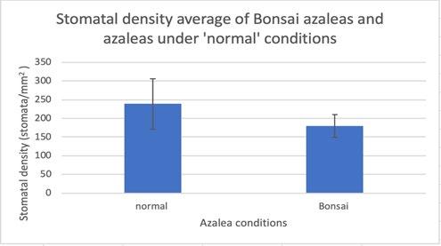
Average Stomatal density (stomata/mm²)
Bonsai conditions 179.5
Normal' conditions 238.5
The results of stomatal density from each leaf were calculated by counting the number of stomata from the 400X field of view and then dividing the number of stomata by the field of view (0.16mm²). This was done for 5 plants under each condition (‘normal’ and Bonsai). Therefore, overall, 10 plants.
From each plant there were 5 sample leaves taken. Therefore, 25 for each condition (50 combined for Bonsai condition and ‘normal’ condition). And one FOV for each leaf was used to calculate the stomatal density of the leaf. Photos that were taken to count the stomata can be seen below in Figures 4 and 5. Once the stomatal density of the 5 leaves from the same plant was calculated then an average of this was calculated to produce the individual plant's average stomatal density. After the average stomatal density was calculated for the 5 plants an overall average was taken to determine the overall average stomatal density for the conditions (i.e. Bonsai or ‘normal’)
Science Extension Journal • 25 Scientific Research in School Volume 4 Issue 1 2022
Discussion
From the five trial plants for each condition the results were gathered and explored. The overall trend indicated that Bonsai azaleas have a lower stomatal density than azaleas grown under ‘normal’ conditions. This appeared to support the hypothesis that azalea plants under Bonsai conditions will have fewer stomata per square mm of leaf than those grown under ‘normal’ conditions. However, statistical tests revealed that there was not a significant difference between the average densities of Bonsaied and ‘normal’ plants. The range of densities from the ‘normal’ conditions was 142.5 stomata/mm² and the range of densities from the Bonsai conditions was 85 stomata/mm². This reflects that the stomatal densities of the plants under ‘normal’ conditions are quite varied more so than the plants under Bonsai conditions. Therefore, the experiment results contained outliers. The experiment could be improved by expanding the sample size however this could not be done due to the
timeframe provided. Therefore, the results were not uniform across all the tests which conveys how the results may be unreliable as the trials may not express the same results if repeated. This may be due to the uncontrolled variables such as the age of the plants and locations of the plants which may contribute to the spread of data. However, standardisation was implemented in the experiment as each sample leaf was picked 5 leaves down from the terminal leaf, the same nail polish and sticky tape was used to collect the leaf imprint, all samples were viewed under a compound light microscope at 400X magnification, and the same person counted the stomata from each leaf.
The key research question was to determine the effect of Bonsai conditions on the density of stomata in azalea plants. This was done by collecting leaves from azalea plants under Bonsai and ‘normal’ conditions. There were 5 trial plants for each condition and 5 sample leaves to gather an average for the plant’s stomatal density. Therefore, there were 25 samples for each condition. The method used to gather the results of the stomatal density included taking an imprint of the underside of the leaf to make the stomata visible to the compound light microscope. Therefore, the method used measured what was aimed using the correct equipment and hence the experiment is valid. The stomata were counted and divided by the field of view (0.16mm²) this gave the stomatal density of the leaf which satisfies the research question. The results from the 5 leaves of the individual plant were averaged to produce the plants average stomatal density. The average stomatal densities of the 5 trial plants for the specific condition were averaged which produced the overall conditions average stomatal density.

Furthermore, if the Bonsai azaleas had a lower stomatal density than azalea plants under ‘normal’ conditions they would have a higher tolerance to drought and increases agricultural productivity under drought conditions (Bertolino and coworkers, 2019). This idea is also supported by Jarvis and Davies, (1997); van Rensburg et al., (1999) and Kleinhenz et al., (1995); Nayeem, (1989) whereby plants with lower stomatal densities may benefit water efficiency under restricted water conditions as they have a higher tolerance to environmental stresses such as drought compared to plants that have higher stomatal densities. However, the results of the experiment cannot determine that the stomatal density is different between azaleas grown under Bonsai conditions and ‘normal’ conditions.

26 • Science Extension Journal Scientific Research in School Volume 4 Issue 1 2022
Figure 4: Imprint of stomata from azalea under 'normal' conditions view from compound microscope at 400X magnification
Figure 5: Imprint of stomata from azalea under Bonsai conditions view from compound microscope at 400X magnification
The differences in morphology such as stomatal density and size arise due to genetic factors and or growth under different environmental conditions (Bertolino, Caine, & Gray, 2019). However, the test signified that the results were not significant and therefore this report cannot claim that the stomatal density has decreased, due to the environmental stress of growth within a limited space.
The key limitations of this study include time constraints which limited the number of samples able to be taken and tested. This reduced the reliability of the results and would be improved if there was a longer period of time which could therefore increase the sample size and reliability of results respectively. If more fields of view could be used to calculate the stomatal density of individual leaves (i.e. 3 FOV for each leaf) the reliability would increase. Also, this report would have been of greater interest to the agricultural sector if it studied the stomatal density of crops under ‘normal’ conditions and Bonsai conditions which could help to compare the efficiency and productivity of crops if they were under bonsai conditions. However, this report by determining the stomatal density of Bonsai azalea plants compared to azalea plants grown under ‘normal’ conditions provides an understanding of the morphology of azalea plants grown under different conditions produce very similar results in respect to stomatal density. Another implication of this study is that there are no other scientific reports which have researched the stomatal density of azalea plants, thus results could not be compared.
In future studies, the plant age and environment should be more consistent to increase the reliability of results. Also, a larger sample size should be taken of each plant and the number of plants tested on as it may indicate the results as significant (i.e. 10 leaves from each plant and 10 plants) as the sample size may be too small to see any differences if there is one. This would also increase the reliability of the report. This paper could also be improved if it could focus on a plant which is used in agriculture and has difficulty growing in drought persistent areas. However, on a high school level, this is difficult to achieve as samples from crops which grow in drought persistent areas would be difficult to access. Further implications of this study include creating crops which are more drought tolerant by placing the crops under Bonsai conditions.
The statistical analysis was done by determining the mean and standard deviation for the Bonsai azalea (M = 179.5, SD = 68.09) and for the azalea under
‘normal’ conditions (M = 238.5, SD = 30.79). Then an independent t test was used to compare the means of the results by inserting the plant trial averages into an online t test calculator which determined the t value (t = 5.58) and P value (P = 0.15). This determined that the results were not significant as P < 0.05. This was very effective at indicating that the data was not significant. However, the sample size used was small and had more than one variable which could have affected the results. Therefore, in further study a larger sample size could further investigate the significance of the experiments results. Also, overall standardisation of the experiment should be implemented to increase the reliability of the experiment.
Although these results are not significant as proven by the data analysis, this study could produce significant results in the future and could help to benefit the growth and production crops in drought persistent regions. The experiment was not reliable because of the outliers in the results however it was valid and accurate because it measured what was aimed and was consistent with other scientific reports. The experiment could have been improved by increasing the sample size, timeframe and implementing further standardisation of the controlled variables. Through this study I found that there is no significant difference between stomatal density of Bonsai azalea plant and azalea plants under ‘normal conditions. However, if the sample size was increased it could provide significant results. Therefore, because stomatal density can determine the rate of water loss it would be advantageous to alter plants to suit the stomatal density to the specific environmental conditions to help plants control of gaseous exchange. Thus, plants stomata could be adapted to suit areas of low water availability by reducing the density of stomata.
Conclusion
Overall, the results obtained provided insight into the varied stomatal densities however showed that the data collected from the trials was not significant. However, further investigation of this topic could increase the sample size and control all variables except the one being tested to investigate whether there is a significant result where P> 0.5. The project tested the research question; the effect of Bonsai conditions on the stomatal density of azalea plants has no significant difference proven by the statistical analysis. The results of the azalea plants under ‘normal’ conditions showed a range of stomatal
Science Extension Journal • 27 Scientific Research in School Volume 4 Issue 1 2022
densities of each plant (i.e. 323.75 stomata/mm² to 181.25 stomata/mm²) with a range of 142.5 stomata/mm² compared to the Bonsai azalea which showed a smaller range of stomatal densities (i.e. 235 stomata/mm² to 150 stomata/mm²) with a range of 85 stomata/mm². The results were not significant; however, the means of the Bonsai azaleas was lower than the azaleas grown under ‘normal’ conditions.
The differences in the azalea’s morphology and more specifically stomatal density are due to the differences in the environmental stresses the plants experience. If there is a lower stomatal density it could help to increase drought tolerance, water conservation and higher levels of soil moisture content of the plant. However, the overall findings are not sufficient to conclude that there is a significant difference in the results of the Bonsai azaleas and azaleas grown under ‘normal’ conditions. This area needs further research with more controlled variables and larger sample sizes to determine whether azalea plants under Bonsai conditions will have fewer stomata per square mm of leaf than those grown under ‘normal’ conditions.
Acknowledgements
I would like to thank Mrs Sarah Cormio and her husband. Mrs Sarah Cormio has inspired me to take on this project. She has been a positive role model and has helped me by providing the Bonsai plants, I could not have done this without her. She also helped me by caring for the Bonsai which I used in my experiment. I also wish to thank my amazing supervisor Dr Terena Holdaway Clarke for helping me continuously throughout this project, she is a great mentor. Finally, I would like to thank the Barker Science Department for allowing me to use the appropriate equipment.
References
Bertolino, L. T., Caine, R. S., & Gray, J. E. (2019). Impact of stomatal density and morphology on water use efficiency in a changing world. Frontiers in Plant Science, 10, 225. https://internal journal.frontiersin.org/articles/10.3389/fpls.2019.00225/fu ll
Casson, S., & Gray, J. E. (2008). Influence of environmental factors on stomatal development. New phytologist, 178(1), 9 23. https://nph.onlinelibrary.wiley.com/doi/full/10.1111/j.146 98137.2007.02351.x
Doheny Adams, T., Hunt, L., Franks, P. J., Beerling, D. J., & Gray, J. E. (2012). Genetic manipulation of stomatal density influences stomatal size, plant growth and tolerance to restricted water supply across a growth carbon dioxide gradient. Philosophical Transactions of the Royal Society B: Biological Sciences, 367(1588), 547 555
https://royalsocietypublishing.org/doi/pdf/10.1098/rstb.20 11.0272
Drake, P. L., Froend, R. H., & Franks, P. J. (2013). Smaller, faster stomata: scaling of stomatal size, rate of response, and stomatal conductance. Journal of experimental botany, 64(2), 495 505.
https://academic.oup.com/jxb/article/64/2/495/531702?log in=true
Hetherington, A. M. (2001). Guard cell signaling. Cell, 107(6), 711 714. https://www.sciencedirect.com/science/article/pii/S00928 67401006067
Kimball, B. A. (2007). Global change and water resources. Irrigation of agricultural crops, 30, 627 653. https://acsess.onlinelibrary.wiley.com/doi/abs/10.2134/agr onmonogr30.2ed.c17
Lawson, T., & Vialet‐Chabrand, S. (2019). Speedy stomata, photosynthesis and plant water use efficiency. New Phytologist, 221(1), 93 98.
https://nph.onlinelibrary.wiley.com/doi/full/10.1111/nph.1 5330
Lawson, T., & Blatt, M. R. (2014). Stomatal size, speed, and responsiveness impact on photosynthesis and water use efficiency. Plant physiology, 164(4), 1556 1570.
https://academic.oup.com/plphys/article/164/4/1556/6112 797?login=true
Passioura, J. B. (2002). Soil conditions and plant growth. Plant, Cell & Environment, 25(2), 311 318
https://onlinelibrary.wiley.com/doi/full/10.1046/j.0016 8025.2001.00802.x
Grant, B. W., & Vatnick, I. (2004). Environmental correlates of leaf stomata density. Teaching issues and Experiments in Ecology, 1(1), 1 24.
https://evoed.evolutionsociety.org/downloads/1170/stomat a.pdf
Xu, Z., & Zhou, G. (2008). Responses of leaf stomatal density to water status and its relationship with photosynthesis in a grass. Journal of experimental botany, 59(12), 3317 3325.
https://academic.oup.com/jxb/article/59/12/3317/627451?l ogin=true
Zhang, Y. I., & Turner, J. G. (2008). Wound induced endogenous jasmonates stunt plant growth by inhibiting mitosis. PloS one, 3(11), e3699. https://journals.plos.org/plosone/article?id=10.1371/journ al.pone.0003699
28 • Science Extension Journal Scientific Research in School Volume 4 Issue 1 2022
Azalea ‘normal’ condition results
Plant Leaf Number of stomata Stomatal density
1 1 25 156.25
1 2 40 250
1 3 30 187.5
1 4 30 187.5
1 5 20 125
2 1 33 206.25
2 2 34 212.5
2 3 29 181.25
2 4 24 150 2 5 26 162.5 3 1 30 187.5
3 2 29 181.25 3 3 28 175 3 4 32 200 3 5 29 181.25
4 1 62 387.5
4 2 38 237.5
4 3 62 387.5
4 4 37 231.25
4 5 57 356.25
5 1 51 318.75
5 2 53 331.25
5 3 46 287.5
5 4 59 368.75 5 5 50 312.5
Azalea Bonsai results
Plant Leaf Number of stomata Stomatal density
1 1 34 212.5
1 2 42 262.5
1 3 35 218.75
1 4 42 262.5
1 5 35 218.75 2 1 34 212.5
2 2 26 162.5 2 3 26 162.5
2 4 37 231.25 2 5 29 181.25
3 1 32 200 3 2 21 131.25 3 3 27 168.75 3 4 22 137.5
3 5 29 181.25 4 1 27 168.75 4 2 21 131.25 4 3 26 162.5 4 4 22 137.5 4 5 31 193.75 5 1 27 168.75 5 2 20 125 5 3 29 181.25 5 4 23 143.75 5 5 21 131.25
Science Extension Journal • 29 Scientific Research in School Volume 4 Issue 1 2022 Appendix
30 • Science Extension Journal Scientific Research in School Volume 4 Issue 1 2022
Concentration of microplastics found in sediment from ocean beaches compared to estuarine beaches in Sydney
Olivia Marlin Barker College
Purpose: This paper aims to seek data on the variance in concentration of microplastics between Sydney's ocean and estuarine environments, indicating areas of a notable concern.
Design/methodology/approach: Twenty four sediment samples were collected from six beaches (three ocean, and three estuarine), and methodologies of density separation and extraction were employed, before conducting a quantitative analysis.
Findings: No evidence of microplastics were identified in this investigation. This was likely due to problems with the methodology adopted. A range of possible errors encountered were explored, as well as four other methodologies that could be used as alternatives for those used in this paper. Each of the alternate methods were evaluated based on the criteria of being suitable for research in schools.
Research Limitations/implications: The methods used were not successful in isolating microplastics from the sand samples collected.
Practical implications: The review of methods for quantifying microplastics that are suitable for use in schools will increase the chance of successful research by students in this area. Individuals will be able to select an appropriate methodology with a comprehensive understanding of its requirements, reducing the chances of encountering methodological errors.
Social Implications: Incorporating a review of methods enables further student and citizen research projects to be successfully undertaken to explore the prevalence of microplastics in sand.
Originality/value: To the author's knowledge, this paper is the first to review a range of methodologies suitable for school research into the prevalence of microplastics in the environment.
Paper Type: Research Paper
Literature Review
Microplastics are small plastic particles less than 5 mm in size. They originate from microbeads commonly used in cosmetic products and microfibres shed from textiles, as well as larger plastic items that have been broken down in size over time, this includes the degradation of single use plastic straws and takeaway containers (Jiang, 2018). Microplastics enter waterways in a variety of ways including human littering, water run off, wind, wastewater, fishing, and shipping activity. Not only is this an issue due to the growing popularity of plastic products, but more so due to the harm that plastics can cause to marine life and ecosystems. The small size and bright colours of microplastics are appealing to fish causing ingestion (Jovanović, 2017). Numerous additives are added to plastic polymers, such as flame retardants, stabilisers and lubricants which cause direct harm to sea life upon digestion and these are further passed on through the food chain, creating issues for entire ecosystems. It has been found that microplastics sorb chemical pollutants that are present in surrounding water, thus creating enhanced toxicity for fish due to them bioaccumulating these pollutants, putting stress on the
liver (Rochman et al., 2013). It is also suggested that consuming an organism that has ingested microplastic may be harmful as the toxic chemicals have been pre absorbed into the organism, indicating that human consumption of fish may also be dangerous (Jovanović, 2017). The existence of microplastics in the food web has been established, but scientists are yet to fully understand what the human health risks will be in the long term.
It is clear microplastics predominantly originate near the coast and remain in a similar area for a long time (Zhang, 2017). In Australia, a current citizen science project has found the presence of microplastic pollution on Australian coastal beaches and harbour side beaches, and early results have shown that Sydney harbour locations have moderate to high levels of microplastics, with some Sydney ocean beaches having lower levels (Wilson, 2022). Influxes of plastic in river systems are a major input of microplastics into marine systems, and rivers have been found to be ‘hotspots’ with a large amount of microplastics found in sediment (Windsor, 2019). A study in China that took samples from both semi enclosed bays and open coastal zones supported this
Science Extension Journal • 31 Scientific Research in School Volume 4 Issue 1 2022
theory as the bays had a greater accumulation of microplastics due to the minimal currents and surrounding topography trapping the microplastics (Sun et al., 2021). On the contrary, a study in Oahu, Hawaii suggested that beaches with higher waves have a greater accumulation of microplastics (Rey et al., 2021). The study concluded that microplastics travel through the ocean, and wave energy increases microplastic density on the shoreline.
Due to Australia having a wide reaching coastline, we are particularly vulnerable to the accumulation of microplastics in both estuarine and ocean environments. A citizen science project conducted across more than 300 beaches Australia wide, has determined that there were over 3 million microplastic fragments found when collecting as part of the Australian Microplastic Assessment Project (Wilson, 2022). It was discovered that, within Sydney, the largest microplastic ‘hotspot’, was Manly Cove, with 4051 microplastics per m2 (“Hotspot Map,” 2015). This poses unease for Sydneysiders, as only a small number of Sydney beaches have been investigated as of present, but those that have, are of notable concern.
Scientific Research Question
Is the quantity of microplastics found in sediment samples in the Sydney region, higher on the shorelines of ocean or estuarine beaches?
Scientific Hypothesis
Sediment samples taken from estuarine beaches in Sydney will have a larger concentration of microplastics, compared to sand samples taken from Sydney’s ocean beaches.
Methodology
The sampling method for this experiment was to take 4 sediment samples from 6 separate locations (24 samples total), which are identified in Figure 1. At each location the first sample, ‘0’, was taken at the water line, then another was taken 1 metre towards drier sand, followed by samples at 2 and 3 metres, represented in Figure 2. Each sample container was labelled with the corresponding location number (1 6), as well as metres from the water (0 3) where the sediment was sampled (e.g. 1.0, 1.1, 1.2, 1.3, 2.0 and so on).
Figure 1: Map of Sydney beaches where samples were collected

Figure 2: Transect line indicating sample collection points
The sand was dried as comparisons of dry mass is much easier, given the varying water content of sand at different distances from the shoreline. 24 glass petri dishes were labelled using the same system as above and laid flat onto large metal trays (see Figure 3). Approximately 25 g of each sample was placed into a petri dish and enough sand was left in the original container to repeat the process later if needed. The samples were placed into an oven at 70oC and were found to be completely dry after 5 hours. Clean sampling containers were labelled using the
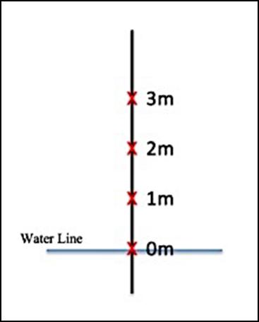
32 • Science Extension Journal Scientific Research in School Volume 4 Issue 1 2022
aforementioned system and the dry samples were individually funnelled into clean containers using a new paper funnel for every sample.
more than 4 mm into the liquid and the tip was situated towards the edge of the container. The liquid extracted, was released onto the clean microscope slide, and covered using a coverslip, before being examined using a light microscope. Each sample was thoroughly inspected and photographed.
Floatation was used to extract the microplastics, following the method of (Prata et al., 2019). This entailed creating a saline solution, which used approximately 190 g of NaCl and 500 mL of H2O to create a saturated solution. Most plastics have a density of 0.90 g/cm3 and a saturated saline solution has a density of 1.202 g/cm3, allowing potential microplastics to float (Hidalgo Ruz et al., 2012). The solution was heated in a glass jar until boiling, while simultaneously being stirred. All possible NaCl was dissolved into the solution and excess settled at the bottom, meaning it was important to not disturb the jar and disperse undissolved NaCl.

24 Centrifuge tubes were labelled according to the previous system and were filled with the dry sand sample to the 4 mL marking on tube. Using a pipette, 4 mL of the previously made saline solution was added to the tubes on top of the sand (see Figures 4 and 5). These samples were vigorously shaken, and then placed directly into a centrifuge for 5 minutes per sample to rapidly settle and separate the sand sample. The machine was set to approximately 2000 RPM (revolutions per minute). The settled samples were then placed into a test tube rack and their movement was kept to a minimum.
Before examining each sample, water was used to determine the volume of liquid that could fit between a microscope slide and a standard size coverslip. An automatic pipette was used to ensure standardisation amongst all sample sizes, and the plastic tip was cut off to create an opening, 2 mm in diameter. 700 µL was found to be the appropriate amount placed onto the microscope slide as it was the maximum amount that did not result in loss of the sample when a slide coverslip was placed on top. When drawing up a sand saline sample, the automatic pipet was submerged no
Figure 4: Centrifuge tube filled with 4 mL of dry sand sample
Figure 5: Centrifuge tube filled with 4 mL of dry sand sample and 4 mL of saline solution

Results
The results of the experiment are as displayed in Table 1, by which each number represents the amount of microplastics identified in the entire sample. No evidence of microplastics were encountered, other than sightings of debris (shown in Figure 6) which were later rejected (as not being microplastics). Had results been found, estuarine beaches (1, 2 and 6) and ocean beaches (3, 4 and 5) would have been averaged and compared, as well as conducting an ANOVA test to further identify whether a significant difference was at hand. Individual averages for each beach would also have been calculated, drawing out trends and variations. Whilst the complete lack of microplastics in the observed samples is unexpected, as it is known microplastics exist in many of these locations (“Hotspot Map,” 2015), the consistency of the data indicates that an error occurred at an earlier stage of the experimental process, such as incorrect extraction.

Science Extension Journal • 33 Scientific Research in School Volume 4 Issue 1 2022
Figure 3: Setup of sand samples for drying before oven
fibres that had come from paper towel and a microfibre cloth when cleaning the microscope slides, seen in Figure 6. To exclude this as data, a trial using paper towel, a microfibre cloth and lint free paper was conducted, whereby clean microscope slides were rubbed with these items and then examined under a microscope. Using the lint free paper as the control, allowed observations to be made that the microfibres were only present after the use of a paper towel or microfibre cloth on the slides, allowing the microfibres to be ruled out as microplastic data.
Discussion of results obtained
experiment was undertaken due to
and dangers
The aim was to identify the environments which contained the highest numbers of microplastics to provide assistance moving forward and limit the expansion of microplastics where possible. The empirical research, as stated in the methodology, undertook multiple trials, and was repeated under various conditions, yet no microplastics were found using the method employed.
An issue that surfaced, which has been briefly mentioned in the results, was the confusion caused by large amounts of debris being sighted upon examining samples under a microscope. Many times, when debris was seen, it was thought to have been microplastics, but upon further research, was excluded. Some of this debris has now been identified as salt crystals due to the saline solution, these are shown in Figure 7. Another item that was commonly found were small
It is also possible that microplastics floating in the brine were not picked up by the pipette extraction method used. Perhaps they were held close to the edge of the centrifuge tube by surface tension and not picked up in the small volume (< 1 mL) used for mounting between a microscope slide and coverslip. Alternatively, the sand samples may have been collected in a manner that meant only a small proportion of the sand collected was taken from the uppermost sediment layer, that would likely contain the most microplastics. As previously stated, microplastics are less dense than seawater, so they are expected to float and accumulate at the high tide line where floating detritus ends up. If the project was to be redone, the protocols of “Guidelines for sampling microplastics on sandy beaches” (Sluka, 2018) would be followed. This would involve sampling from only the high tide line and using a transect along this, rather than vertically from the sea towards drier sand. Samples would also be only collected from the top 5 cm of sand, possibly using a quadrat. Sand samples would be collected in larger amounts, then followed by a methodology to concentrate the microplastic particles, such as floatation in brine and straining by filter paper (Besley et al., 2017).


34 • Science Extension Journal Scientific Research in School Volume 4 Issue 1 2022 Table 1: Results of microplastic findings (units in quantity per sample) Beach Count of microplastics 0m from water line 1m from water line 2m from water line 3m from water line 1 0 0 0 0 2 0 0 0 0 3 0 0 0 0 4 0 0 0 0 5 0 0 0 0 6 0 0 0 0 Figure 5 : Debris observed through microscope Discussion
This
increasing rates
surrounding microplastics.
Figure 6: Square particles are salt crystals observed through microscope
Review of methods for visualising microplastics suitable for use in schools
The results of this study show that isolation and visualisation of small microplastics from sand samples is not an easy task. As microplastics are a growing problem, and the magnitude of the task of surveying the world's beaches is well suited to a citizen science approach (note the AUSMAP site which does citizen science for microplastics “Hotspot Map,” 2015), a survey of the current literature was conducted. This reviewed a range of methods for visualising microplastics in sand samples that would be suitable for use in schools. A summary of the methodologies is given in Table 2.
Sieving using density separation

This method (Kunz, 2021) is used to initially separate microplastic particles from sand. It consists of first conducting a density separation, using a saturated salt solution (NaCl), whereby the solution has a density of 1.2 g/cm3, allowing microplastics to float as they have a lower density. This solution is added to a beaker along with the dry sand sample, stirred, and then the supernatant is poured through sieves of decreasing sizes, as seen in Figure 8, separating the sample's particles into different size classes. Concentrated ethanol is then used to separate the solution, by which ethanol has a density of 0.789 g/cm3 causing the majority of the plastics and heavier materials to sink to the bottom. The remaining sample from the previous separation is combined with the ethanol, stirred and the supernatant is strained, leaving two fractions of lighter and heavier materials. The two fractions will contain pieces of driftwood which have a density of about 1.5 g/cm3 but will always float due to air in its pores, thus, a vacuum pump is used to remove airspace allowing the driftwood to sink, leaving only plastic particles floating in the two samples (and driftwood at the bottom), as seen in Figure 9. The remaining samples can then be poured off and examined. A video of this method is available (Microplastic Research Taiwan, 2021). This method is optimised for sand samples that contain high amounts of driftwood and other organic material and aimed to extract larger microplastics by providing samples free of excess material that can be easily examined. The specific sizes of microplastics were not identified but were categorised as; mostly fragments with small amounts of wood or foamed plastic and, mostly styrofoam with small amounts of fragments or wood (Kunz, 2021). Additionally, this

method is inexpensive and allows effective separation of a sample within a school research environment.
Filtration
Decanting a larger volume of liquid and filtering it through filter paper has been shown to be effective when extracting microplastics from a solution (Besley et al., 2017). This method first requires a density separation, in which a sand sample is added directly to a supersaturated solution and swirled, causing light weight particles, such as microplastics to float. By filter paper (for larger microplastics) or very fine mesh (for very small microplastics), the surface liquid of the mixture is strained, ensuring only the supernatant (containing the lightweight particles) is poured off and denser particles such as sand or undissolved salt do not wash onto the filter paper. The filter paper (or fine mesh) can be observed under a dissecting microscope, whereupon microplastics can be examined and quantified. In a trial conducted of this methodology, microplastics were detected (as seen in Figure 10), in which all were <1 mm in diameter and the smallest being approximately 10 μm.
This methodology provides reliable extraction of microplastics from a solution so that they can be easily examined after separation from a sample. It is effective when conducting research within schools as the equipment is cheap and easily accessible, and the methodology does not contain multiple steps, nor is it
Science Extension Journal • 35 Scientific Research in School Volume 4 Issue 1 2022
Figure 8: Separated sample Source: Microplastic Research Taiwan (2021)
Figure 8: Sieving sample Reprinted from Microplastic Research Taiwan, (2021) Sieving sample Reprinted from Microplastic Research Taiwan, (2021) 7: Sieving sample Source: Microplastic Research Taiwan (2021)
complex. Filter paper has been shown to successfully detect microplastics as small as 100 μm in diameter (Zhu et al., 2020), supporting that there is very little sample lost in the extraction phase. The filter paper may also be replaced with a very fine mesh (At present the smallest available being 2.5 μm), allowing the investigation to be tailored to detecting a variety of microplastic size ranges. Problems include sand getting in the sample, which does obscure results, but rinsing the edge of the tube with the brine, prior to decanting, or pipetting out the supernatant would significantly reduce contamination by sand.
microplastics must be highly concentrated or separated from their sediment sample before being stained with NR. Many reports have stated that a density separation is best for this process (Maes et al., 2017), but others outline that sieving may also be used, in which the sample is poured through sieves of 5 mm, 1 mm, and 0.3 mm (Foster et al., 2015). Once microplastics are isolated, they are treated with NR, which is used at an optimum concentration of 10 μg/mL, (Maes et al., 2017). The dye then must be excited using an LED light source for fluorescence detection.
Figure 9: Microplastics observed under microscope. A clear plastic ruler with mm marks is in each FOV. (Source: Taylor, 2022)

Staining of microplastics with fluorescent dyes
Many studies on small microplastics (which were the target of this investigation) have involved staining with a fluorescent dye. Nile red (NR) is a lipophilic dye that efficiently stains microplastics (Shim et al., 2016) as it is a hydrophobic fluorophore that binds to neutral lipids and is strongly fluorescent whilst in a hydrophobic environment (Nie & Stürzenbaum, 2017). Fluorescence microscopy follows the principle that when the microplastic specimen is illuminated with a light of a specific wavelength, it is absorbed by the fluorophores and will result in the microplastics emitting light of a different, longer wavelength. Nile Red may be excited by blue or green light and emits in the orange red part of the spectrum (See Figure 11). An orange filter may be used to let only the emission wavelength pass through, and not the exciting wavelengths.
Investigations that utilise this method consist of first conducting a process of extraction, whereby
Traditional fluorescence microscopes are too expensive for use in schools (at least $4500 “Optico N300F LED Fluorescent Microscope,” 2018) but there are some simple ways to convert a regular school microscope into an instrument that can view fluorescent dyes. A range of bright field microscopes have been tested for their suitability for adaptation to fluorescence detection, and it has been determined that any stereo and most compound microscopes operating up to 100x magnification can be adapted (Labbe, Bagshaw and Uttal, 2020). In this economical method, the excitation wavelength for NR fluorescence is provided by a blue (450 nm wavelength) LED flashlight, in which another lens taken from an identical LED flashlight was attached to the existing lens, allowing the LED chip to be focused to a 2 mm square. The flashlight is held at an angle of 40° to 60° to the sample and a small yellow filter is attached to the objective lens. An in depth description of this setup is available in a video (Bagshaw, 2019). This adaptation utilises materials that are both inexpensive and easily accessible, making it suitable to be carried out in a school setting, whilst still providing high quality results.

36 • Science Extension Journal Scientific Research in School Volume 4 Issue 1 2022
Figure 10: Nile Red excitation is shown in dotted line, emission in solid shading (Source: Fluorescence SpectraViewer)
Table 1: Summary of methodologies for viewing microplastics in sand samples based on suitability for use in schools
Problem addressed Positives Negatives
Sieving using density separation (Kunz, 2021)
A more foolproof method for separation of microplastics from sediment samples
Effectively separates sample into multiple size classes Optimal for samples containing high amounts of organic material Inexpensive
Designed for extracting larger microplastics Involves multiple steps
Filtration (Besley et al., 2017)
Traditional purpose built fluorescence microscopy
(Maes et al., 2017)
Budget fluorescence microscopy (Labbe, Bagshaw and Uttal, 2020)
Video setup: (Bagshaw, 2019)
Allows successful extraction of microplastics after separation
Shown to have very little sample loss in extraction phase
Inexpensive and accessible materials
Simple methodology
Able to detect microplastics as small as 100 μm in diameter, and can be tailored to different size ranges
May not separate sample as effectively as other methods
Highly effective detection of microplastics when examining
Allows clear visibility of microplastics Commonly used method across eminent microplastic investigations
Very expensive equipment
Requires complex steps Nile Red dye requires sourcing through specialist suppliers
Highly effective detection of microplastics when examining
Made inexpensive by modifications to school laboratory compound microscopes or dissecting microscopes
Majority of equipment is easily accessible and can usually be sourced through school
Allows clear visibility of microplastics
Requires additional set up Nile Red dye requires sourcing through specialist suppliers
Conclusion
The investigation carried out did not identify any microplastics in the samples collected, thus no conclusion could be drawn as to whether the microplastic numbers found in sediment samples from the Sydney region were higher on the shorelines of ocean beaches, or estuarine beaches. The reason for no data being evident was most likely due to flaws in the methodology, or more specifically in the sampling, separation, extraction or examining processes. Due to this, we cannot yet accept or reject the stated hypothesis, as we can argue that the samples collected
may have contained microplastics, but these could not be identified with the method used.
To provide a basis of furthering research on the subject matter, numerous alternate methodologies of extracting and quantifying microplastics have been identified and evaluated. Each methodology was reviewed based on the criteria of being suitable for use in schools. The literature review of methods for inexpensive isolation of small microplastics will allow future researchers to be aware of problems that may arise, and additionally utilise the suggestions made
Science Extension Journal • 37 Scientific Research in School Volume 4 Issue 1 2022
Technique
when carrying out their surveys on microplastic levels on beaches.
Acknowledgements
Thank you to Dr Alison Gates who helped to come up with a new approach to my project and talked me through how I would reconstruct each section. To Mrs Nonie Taylor for offering her assistance and providing information on the filtration method. To Dr Matthew Hill for lending guidance wherever possible. And a special thank you to Dr Terena Holdaway Clarke who supported me through my research process, reassuring me when I could not find data and constantly giving feedback on my report.
References
Bagshaw, C. (2019). 01262 Nile Red fluorescence [YouTube Video]. Retrieved from https://www.youtube.com/watch?v=BYvU9sOAuFM&t=1 s
Besley, A, Vijver, MG, Behrens, P & Bosker, T 2017, ‘A standardized method for sampling and extraction methods for quantifying microplastics in beach sand’, Marine Pollution Bulletin, vol. 114, no. 1, pp. 77 83, viewed 18 June 2022, <https://www.sciencedirect.com/science/article/abs/pii/S00 25326X16306877>.
Fluorescence SpectraViewer. (2020). Retrieved June 8, 2022, from Thermofisher.com website: https://www.thermofisher.com/order/fluorescence spectraviewer?SID=srch svtool&UID=1142gto#!/?SID=srch svtool&UID=1142gto Foster, G., Mausra, Baker, Foster, & Arthur. (2015). Photo credit: NOAA Marine Debris Program Laboratory Methods for the Analysis of Microplastics in the Marine Environment: Recommendations for quantifying synthetic particles in waters and sediments. Retrieved from https://marinedebris.noaa.gov/sites/default/files/publication s files/noaa_microplastics_methods_manual.pdf
Hidalgo Ruz, V., Gutow, L., Thompson, R., & Thiel, M. (2012). Microplastics in the Marine Environment: A Review of the Methods Used for Identification and Quantification. ACS Publications, 46(6). Retrieved from https://pubs.acs.org/doi/abs/10.1021/es2031505
Hotspot Map. (2015). Retrieved June 18, 2022, from Ausmap.org website: https://www.ausmap.org/hotspot map
Jiang, J. Q. (2018). Occurrence of microplastics and its pollution in the environment: A review. Sustainable production and consumption, 13, 16 23.
Jovanović, B. (2017). Ingestion of microplastics by fish and its potential consequences from a physical perspective. Integrated environmental assessment and management. 13(3), 510 515.
Kunz, A. (2021). Microplastic Research in Taiwan. Retrieved June 17, 2022, from Microplastic Research in Taiwan website: https://microplasticresearch.wordpress.com/
Labbe, A. B., Bagshaw, C. R., & Uttal, L. (2020). Inexpensive Adaptations of Basic Microscopes for the Identification of Microplastic Contamination Using Polarization and Nile Red Fluorescence Detection. Journal of Chemical Education, 97(11), 4026 4032. https://doi.org/10.1021/acs.jchemed.0c00518
Maes, T., Jessop, R., Wellner, N., Haupt, K., & Mayes, A. G. (2017). A rapid screening approach to detect and quantify microplastics based on fluorescent tagging with Nile Red. Scientific Reports, 7(1). https://doi.org/10.1038/srep44501
Microplastic Research Taiwan. (2021). Microplastic extraction from beach sediments [YouTube Video]. Retrieved from https://www.youtube.com/watch?v=W8mLqxpzW0o&t=5s
Nie, Y., & Stürzenbaum, S. R. (2017). Model Nematodes in Obesity Research. Animal Models for the Study of Human Disease, 267 280. https://doi.org/10.1016/b978 0 12 809468 6.00011 5
Optico N300F LED Fluorescent Microscope. (2018). Retrieved June 19, 2022, from Microscopes.com.au website: https://microscopes.com.au/products/optico n300f led fluorescent microscope?_pos=1&_sid=186be1cfb&_ss=r
Prata, J. C., da Costa, J. P., Duarte, A. C., & Rocha Santos, T. (2019). Methods for sampling and detection of microplastics in water and sediment: A critical review. TrAC Trends in Analytical Chemistry, 110, 150 159. https://doi.org/10.1016/j.trac.2018.10.029 Rey SF, Franklin J, Rey SJ (2021). Microplastic pollution on island beaches, Oahu, Hawai`i. PLOS ONE 16(2): e0247224
Rochman, C. M., Hoh, E., Kurobe, T., & Teh, S. J. (2013). Ingested plastic transfers hazardous chemicals to fish and induces hepatic stress. Scientific Reports, 3(1). https://doi.org/10.1038/srep03263
Shim, W. J., Song, Y. K., Hong, S. H., & Jang, M. (2016). Identification and quantification of microplastics using Nile Red staining. Marine Pollution Bulletin, 113(1 2), 469 476. https://doi.org/10.1016/j.marpolbul.2016.10.049
Sluka, R. (2018). Guidelines for sampling microplastics on sandy beaches. Retrieved from https://www.arocha.org/wp content/uploads/2018/01/Microplastic sampling protocol.pdf
Sun, X., Wang, T., Chen, B., Booth, A. M., Liu, S., Wang, R., & Xia, B. (2021). Factors influencing the occurrence and distribution of microplastics in coastal sediments: From source to sink. Journal of Hazardous Materials, Volume 410, 124982
38 • Science Extension Journal Scientific Research in School Volume 4 Issue 1 2022
Taylor, N. (2022, May). New method of filtration for microplastics in sand, using filter paper [Letter to Terena Holdaway Clarke; Face to face].
Wilson, S (2022). You know you’re swimming in it worst beaches for swimming revealed. The Lighthouse, Macquarie University.
Windsor, F. M., Durance, I., Horton, A. A., Thompson, R. C., Tyler, C. R., & Ormerod, S. J. (2019). A catchment scale perspective of plastic pollution. Global Change Biology, 25(4), 1207 1221
Zhang, H. (2017). Transport of microplastics in coastal seas. Estuarine, Coastal and Shelf Science, 199, 74 86. https://doi.org/10.1016/j.ecss.2017.09.032
Zhu, C., Kanaya, Y., Nakajima, R., Tsuchiya, M., Nomaki, H., Kitahashi, T., & Fujikura, K. (2020). Characterization of microplastics on filter substrates based on hyperspectral imaging: Laboratory assessments. Environmental Pollution, 263, 114296. https://doi.org/10.1016/j.envpol.2020.114296
Science Extension Journal • 39 Scientific Research in School Volume 4 Issue 1 2022
40 • Science Extension Journal Scientific Research in School Volume 4 Issue 1 2022
The importance of fungi investigation in the effect of cellulase enzymes on the growth rate and fungal spore density with Pleurotus ostreatus
Sam Young
Barker College
Purpose: The purpose of this paper is to provide a new growth accelerant in fungal growth, specifically oyster mushrooms as to find the effect of the enzyme cellulase on the growth and sporification density and production of oyster mushrooms. This in which is to find new and faster ways to grow oyster mushrooms and fungi for both agricultural and industrial use.
Design/methodology/approach: The experiment used a substrate mixture of hydrated lime (250 ml) mixed with 5kg of sugarcane mulch inoculated with Pleurotus ostreaus oyster mushroom breed of spawn, distributed in 10 mushroom bags. Once the pinhead stage occurred the mushrooms bags were cut to allow for growth of oyster mushrooms outside of the bag, and 4 were chosen to be sprayed with diluted cellulase (diluted in distilled water) (9 sprays per bag) and 4 were chosen to be controls through size and length of mushroom being paired with similar pairs. The weight of the bags was measured every 5 days and after the 15 days mark the 5 mushroom caps or caps from the test were cut and put on a piece of paper to produce a spore print. (figure 2).
Findings: The research found that the synthetic introduction of the cellulase enzyme caused an increase in both growth rates (seen through larger weight percentage reduction in the mushroom bags). This partnered with the higher density and yield of the spore prints with the introduced cellulase.
Research limitations/implications: The paper was limited to one specific breed of mushroom as well as only having a sample size of one enzyme dilution for the cellulase (5 ml of cellulase per 200ml of distilled water). In future tests more trials can be conducted, as well as the tests with different oyster mushroom breads rather than just PO and using different dilutions of cellulase.
Practical implications: The results showed a clear indication for the use of cellulase to help stimulate and increase both the growth rates, spore density, and spore yield. In which provides a new stimulant for oyster mushroom growth.
Social implications: The results of the findings can be used to understand and develop new growing techniques in both fungal spores and growing of edible oyster mushrooms.
Originality/value: To the knowledge of the researcher, the use of synthetic introduction of any enzyme to see the effects of anything on mushrooms, nor has there been any recording of the effect of the introduced cellulase enzyme on growth rate of oyster mushrooms and fungal spore yield.
Keywords: Growth rates, Fungal spores, Spore density.
Literature Review
Importance of mushrooms to humans
Mushrooms have been consumed by humans for as long as human recorded history, its first recorded use hundreds of years BC, as shown in the roman times to be perceived as the “food of the gods” (Valverde et al, 2015). They have also been shown to have a large health benefit showing attributes of anti cancerous, anti cholesterol, anti allergenic properties as well as showing aspects of rich in carbohydrates like, chitin, hemicellulose, beta, and alpha glucans, mannans, xylans, and glycans for most farmed edible mushrooms (Jayachandran et al, 2017). Due to their dietary ability, mushrooms can provide a clear substitute for products harder to grow or have a
longer turnover rate such as beef or cattle for the food shortage crisis leaving 800 million hungry (DeRose et al, 1998). The importance of mushrooms and their turnover rate of most edible mushrooms like oyster mushrooms being 21 28 days (Sharma et al, 2013).
The use and importance of mushrooms can be seen in the recent mushroom cultivation and farming as one of the largest agricultural areas, however, is shown to have to combat supply increase of 30 fold worldwide from 1978 to August the 14th 2017, this in which has mainly increased in the 21st century due to the investigation of medicinal benefits and a renewable substitute for products that use more resources (meat) (Royse et al, 2017).
Science Extension Journal • 41 Scientific Research in School Volume 4 Issue 1 2022
K. Piska al (2017) furthers these ideas of nutritional value and ability of mushrooms specifically Pleurotus Ostreatus (PO), as being the most soled oyster mushrooms across all continents except Antarctica. Investigating the possible abilities and nutritional values it may hold for further use, demonstrating the richness in primary and secondary metabolites. showing that only 100 grams of the fresh fruiting bodies can give 15% of the recommended daily intake of vitamin C, 40% of niacin, riboflavin, and thiamin, and 0.5 mg of vitamin B12. This species is also characterized by a high content of oleic acid (40%), linolenic acid (55%). Emphasising its ability and use in areas of medicine, agriculture, and food showing a clear indication of use for healing and restoring civilisation diseases, such as diabetes. He in which explains how the use of PO can be shown in many areas, demonstrating its ability to grow in harsher climates and use less resources for the same product when comparing to meat or other fruits. He shows the ability for PO to be developed in uses beneficial to humanity such as the ability to grow in harsh environments and the ability to develop amounts of vitamin c in a shorter growth period. Hence the ability mushrooms provide to humanity can be seen in the abilities PO is able to give, thereby showing its importance through its abilities that benefit humanity indicating further research in cultivation, production, and abilities demonstrating the benefit of edible mushrooms to humanity and thereby its importance.
Mushrooms (PO) physiology and effects of environmental and chemical changes on it Mushroom physiology mainly refers to the nutrition, metabolism, growth, reproduction and death of fungal cells (GM Walker, et al). Fungal cells like any generally will rely and depend upon the biotic and abiotic factors that are in their necessary environment. When specifying with the tested mushroom (oyster mushroom (PO), it is found that the mushroom physiology is more structured and is formed to be much largely collected to the environment, showing that when the mushroom is put in a different temperature and container it was shown to have significant effects on the respiratory rate solubility and water content (Rajarathnam et al., 1983). The further effectors of the PO’s physiology are further shown chemically through chemicals such as oxygen and nitrogen synthetically added within the actual system showing a significant change in growth rate with synthetic introduction (Liu, Z et al., 2010). Therefore, showing that both chemical and physical environmental factors will affect the overall health
and quality of the product it is clear to see that the effect of mushroom size and growth is affected both chemically and environmentally. The second factor is also the negative indication of certain chemical changes (seen in fig 1) both temperature and moisture level can affect the growing as well as the decay of the oyster mushroom. Oyster mushrooms and fungi are both effected ab y environment and chemical factors there by the testing should be further based on the effects of the changes of environment or chemical concentration change.

Figure 1: The effect of environmental water change and its dehydration with oyster mushrooms
Identification of a research gap
There is limited research in a large factor of the biotechnology of enzyme production with relation to production rates (such as phosphorylase and cellulase). Indicating that the point of research gap, indicated through the lack of enzyme experimentation on both the qualitative growth and consumption rate of the substrate as well as the spore yield and density. Hence the purpose of this experiment is to investigate this, in which it hopes to see if there is an effect in the growth rate and spore density when it is synthetically introduced with cellulase, providing information in whether this could be used as a viable biotechnology in growing mushrooms more efficiently
Figure 2: Mushroom life cycle

42 • Science Extension Journal Scientific Research in School Volume 4 Issue 1 2022
Scientific Research Question
What is the effect of synthetic introduction of the cellulase enzyme on the fungal spore density, observable characteristics, and overall growth rate of oyster mushrooms?

Scientific Hypothesis
Primary: The introduced cellulase enzyme will increase the fungal spore density, indicated by the higher density and colouration of the spore print.

Secondary: The growth rate of the oyster mushrooms will increase with the introduced cellulase, indicated by the higher percentage of weight loss in the mushroom bags containing cellulase.
Methodology
Experimental design
The experiments were conducted in the science extension lab at Barker College in the winter of 2022 (May to June). The experiments were arranged in a randomised complete design with 4 replications per test.
Before starting the experiment, safety equipment was worn, such as gloves and eye protection as well as a mask (prevention of contamination control), as well as priming two large jugs of 10L capacity heating the water over pasteurisation temperature (80C), this also included the buying of cellulase solution from sigma Store.
Pasteurisation of substrate
The sugar cane mulch was put in a 50 litre capacity esky in which it was wet down with water (approximately 8 litres). In which afterward 250 millilitres hydrated lime was carefully added on the top of the mixture. The hydrated lime was mixed into the substrate until completely dissolved (cannot see hydrated lime powder). In which the substrate hydrated lime mixture was then put evenly in two separate pillowcases to strain the water. In which place both pillowcases in a suitably sized esky that can fit the two pillowcases comfortably (pillowcases can fit without any added pushing or force rather than closing the lid). In which once the water reached 80C by the jug, the water was then poured in the esky with the pillow cases until the pillow cases where fully submerged. Once the pillowcases were fully submerged the esky was then closed. After 2 hours the esky was then opened in which each pillowcase was then moved to a sink to then drain. One drained the pillowcases of substrate where then moved to an unstainable tabletop in which the substrate was then taken out of the bag and onto the table and spread out around the table to cool to at around 35 degrees celsius. The substrate was then spread out along a sterilised bench top (about 3 inches of substrate depth).
Setting up for the growing of mushrooms
The growing of the mushrooms consisted of the materials said above. 5 kg of sugar cane mulch was sterilised in a hydrated lime solution in which was placed in the solution for 2 hours. After which the mulch was put in 10 separate sterile spawn bags (evenly) in which the mulch was then settled in the bag. That in which the oyster mushroom fungal spores were then placed on a separate equal container. This in which was then weighed to make sure each container contained the same number of fungal spores (controlled). Each container of spores was then put into the mulch filled spore bags and then mixed through evenly (mixed with gloves on to prevent contamination through oils of hands).
Science Extension Journal • 43 Scientific Research in School Volume 4 Issue 1 2022
Figure 3: A mushroom spore print
Figure 4: mushroom spore print example
Inoculation of the substrate
Taking the bag of the broken up spawn, it was then sprinkled along the length of the cooled substrate until spawn is used and evenly distributed in the substrate the substrate was then mixed well (to ensure even distribution of spawn in substrate control). In which the inoculated substrate was then put into mushroom bags (5 handfuls per bag), then put under the sink with constant temperature.
Setting up greenroom environment
The green room was sterilised and cleaned using alcohol wipes. Ensuring that the temperature was approximately 25 28 degrees (as is the optimum temperature), an automatic humidity sensor dispensing water vapor every 4 minutes was introduced. In which once the spawn showed the visual development of the hyphal knot stage, the mushroom bags were then put in the greenhouse environment.

Cutting the mushroom bags
Once there was visible indication of the next phase of the fungal growth and development (pinhead stage seen in fig 5). The bags were cut with 4cm length crossing directly above the pin head areas. lines to allow for growth outside of the mushroom bags, in which after 5 cuts were made on each bag, they were then put back in the green house until about a 2 cm of full body mushroom growth was found in each bag.
Mixing cellulase solution
Gloves were worn throughout dealing to prevent contamination with oils as well as breather directly over it was prevented to also prevent contamination of the cellulase and the substrate. The cellulase solution was removed from a refrigerator unit whilst still in the bag and was then put in a ratio 0f 5ml of cellulase per 200ml of distilled water. This in which the mixed solution was put in a spray bottle and then refrigerated until use.
Post oyster mushroom fruiting
Once each mushroom bag had oyster mushrooms over 2 cm in length, the mushroom bags were matched with similar size and shape of the developed mushroom outside. This in which each paired bag was separated to a control group and a test group either test a or b was random choice as the container could only fit two and there were four containers).
Everyday afterwards, the diluted cellulase was then sprayed on the test mushroom bags (TMB).
Spore printing
After a three week period of the mushrooms being sprayed with the enzyme solution, the oyster mushroom was then cut 0.5cm at the stalk from the pileus in which was then placed gills down in the center of a black piece of paper this in which each piece of paper with the mushroom was then covered with a sterilized container (sterilised using pasteurization).
Data analysis
Mushrooms were cut (same amount cut from each bag 1). Each mushroom was put on a piece of paper (the paper was marked as either control or test, test was the mushrooms with the introduced cellulase, and control was the mushrooms without introduced cellulase). Each mushroom was given a number to identify both the mushroom and their spore print (seen through figure 4 as an example of a spore print) Spore prints were measured qualitatively out of ten, in which the mushroom with the largest spore prints were given a score of 10 (10 being the largest spore print and 1 being the smallest). This similarly to the spores developed on the mushrooms itself and the way they were measured (10 being the largest number of developed spores on the mushroom, and 1 being the lowest developed spores on the mushrooms). However, the bag weight was measured quantitatively over a 15 day period and weight was recorded every 5 days (measured in grams).
44 • Science Extension Journal Scientific Research in School Volume 4 Issue 1 2022
Figure 5: pin head stage of mushroom development
Discussion and Results
Table 1: Bag weight loss over 15 day period C= control, T= test, N= not used in experiment. (1 or 2 is group)
Bag number Group (TCN) Weight (g) Day
Weight (g) Day
Weight (g) Day 10
Weight (g) Day 15
Weight Loss (g) Day 15
Percentage Weight Loss (%)
1 C1 1071.63 993.6 983.5 976.52 95.11 8.8
3 T2 910.41 870.26 820.66 790.25 120.16 13.2
5 N 875.02 820.94 806.92 782.13 92.87 10.6
6 C2 779.2 753.45 732.93 718.61 60.59 7.8
7 C1 959.41 923.46 903.83 873.73 85.68 8.9
8 C2 841.58 809.93 788.5 765.13 76.45 9.1
9 T2 1002.19 930.67 907.98 866.67 135.52 12.5
10 N 941.51 905.63 880.57 829.91 111.6 11.9
Mushrooms require basic food and other nutrients to grow. Oyster mushrooms are no exception. To cultivate and grow oyster mushrooms in a laboratory, the compounds and nutrients must be provided for their growth and other life processes. In the current study a specific strain of oyster mushrooms (PO) was successfully grown to whole body mushrooms in the laboratory scenario.
The experimental design was based on the idea of both the many testable features of mushrooms in the experiment such as weight spore density. This partnered with the large range and use of both the qualitative and quantitative data that will be retrieved i.e., the spore print and spore density as well as the bag weight (quantitative). This in which caused the creation of the secondary hypothesis of bag weight to then provide other forms of data showing the benefit of the use of cellulase. Another influence in the experimental design
Due to the mushrooms only being able to take nutrients through the mushroom bags, the mushroom growth rates were recorded with the weight loss from the mushroom bags. This is due to the mushrooms structure, being their use of aerobiotic respiration meaning that it releases waste in air and ground. This is due to the fungi’s myselial structure in which all fungi and mushrooms share in which is used in the mushroom anatomy to then make the nutrients into a nutrient rich liquid which then can be more efficiently absorbed this in which is then secreted from. In which the then waste of the liquid is both evaporated and secreted outside of the mushrooms as well as inside PO’s environment to then be re absorbed. Their process of aerobic respiration as well as require nutrients for other chemical and cellular reproduction (e g , mitosis) and release waste and other products throughout the growth cycle due to the chemical processes, the bag's overall weight will be reduced as no new substrate is being added. The mycelium
absorbs the sugar cane mulch for nutrients for their chemical processes. The mycelium/mushrooms produce waste with their chemical processes. Products from the waste can only originate from the substrate (due to the only nutrients available for the mushrooms in the mushroom bags being the sugarcane mulch substrate). It was consuming the nutrients from the sugar cane mulch and releasing waste products outside the bags. During the investigation, half the mushroom bags were sprayed with diluted cellulase enzymes (5mL of cellulase per 200mL of distilled water sprayed nine times) to identify its effects on the mushroom's growth rate and sporification yield.
Data from Table 1 and Figure 4 showed a weight loss difference between the oyster mushrooms sprayed with cellulase and without (an average 30 gram weight difference between the two). The average weight reduction between the control mushroom bags (CMB) and the test mushroom bags (TMB) ranged between 60.59 and 135.52 at 15 days after the spraying of cellulase was initiated. The mushrooms sprayed with cellulase showed an apparent higher weight reduction, CMB showed an average of 8% weight loss compared to a TMB showing an average of 12%. (table 1 fig 4) This is due to the mushrooms with introduced cellulase having a significantly higher ability to break down sugars faster as they have a higher count of cellulase enzymes in the mushroom body. As indicated similarly by B. Adney and J. Baker (2008) [6], cellulase concentrations were able to break down glucose concentrations. Indicating that higher amounts of the enzyme (cellulase) were able to break down the quantities of glucose faster. Showing cellulase breaks down the glucose. As well as showing similar results to Meidute, S., et al (2008) showing results of increase in respiration and absorption of complex carbon sources like glucose or enzymes, showing the effect of it through respiration being tenfold for the
Science Extension Journal • 45 Scientific Research in School Volume 4 Issue 1 2022
0
5
mushroom with introduced complex carbon sources to the control.
Effect of introduced cellulase on the spore density with both the spore print and spores on mushrooms.


Fungal spores are shown to be a vitally important aspect of growing any mushrooms. It is like a seed of a plant. The research investigated the effect of the introduced cellulase on the oyster mushrooms' spore production, density. This in which was measured using the same CMB and TMB mushrooms. The mushroom caps were cut on day 15 from both CMB’s and TMB’s. The cut mushroom caps left on spore paper for three days. In which the TMB caps showed a clear indication of more densely packed with spores (table 2 and fig 5), as shown with the scoring system (described in the method). The TMB oyster mushrooms showed a clear indication of higher spore density on the mushroom and on the spore paper (table 3 and table 2). The score was shown to be an average of 3 for the CMB caps section and an 8 for the TMB caps for the spores on the mushrooms. They also showed that the TMB caps had a much faster and higher density of spores produced on the spore paper on the mushrooms than CMB over the three days showing visible spore prints on the first day, except for one case. This in which the qualitative measurement showed a similar difference being on average for the CMB to be 5/10 and the TMB caps spore score to be an 8/10. Initially, this was considered the result for the question. As cellulase was demonstrated as one of the leading products in mushroom spores’ pre germination (1x10 3 units of cellulase per spore) (Hagerman et al 1985).
The growth rate in both cases can be seen with the large differences in the weight loss percentage averages with the CMB and TMB, showing a 4% difference (30 grams difference as an average) and the spore scores tests, which indicates higher density and yield (spore paper test score 8 whilst control score 3). This directly supports the hypothesis as it indicates that the use of cellulase can be used to increase both the growth rate (seen in Figure 9) of the mushrooms and the spore density.

Figure

46 • Science Extension Journal Scientific Research in School Volume 4 Issue 1 2022
5:
column graph weight loss per bag over the 15 days as well as the test section and control average
Figure
6:
Column graph of all the percentage weight losses averages.
Figure 7: Spore prints of mushrooms
Table 1: Spore print ranking test and control data Spore print number Score out of ten (1 smallest spore print 10 largest)
Test 1 4
Test 2 10
Test 3 8 Test 4 9 Test 5 6 Control 1 1 Control 2 2 Control 3 3 Control 4 7 Control 5 5
Figure 8: The spores developed on the mushrooms as shown. The number indicating the specific mushroom cap.
Table 2: Spores developed on the mushrooms measured qualitatively and given scores for each Mushroom number Scores
Test 1 6
Test 2 9
Test 3 8 Test 4 10 Test 5 7 Control 1 4 Control 2 5 Control 3 1 Control 4 3 Control 5 2
Further research
More research should be conducted on the complete mushroom life cycle to show more in depth findings on the effect of cellulase on the spore yield, density, and growth rate. In addition, a greater variety of mushroom breeds and amounts of cellulase concentrate to distilled water would deepen the research. Combined with more accurate equipment, such as a constant stable temperature environment in a controlled greenhouse and a more accurate humidifier to have a more constant humidity percentage should be considered for further research.

Conclusion
Figure 9: On the left is the control and on the right is the test as shown much larger amounts of stems and larger in size for the test group
Limitations
The experiment's limitation is mainly introduced by the lower amounts of repetition, only having four for each case (being the control and the tests). This means the issue of repetition may challenge. This partnered with the reduced repetition of only using 5 for both tests and controls causes an issue with reliability as the five may have been outliers.
The results supported the primary and secondary hypotheses. The primary hypothesis stated that the introduced cellulase enzyme would increase the fungal spore yield, indicated by the higher density and colouration of the spore print on paper as well as the spore growth of the mushroom itself. This is seen clearly through the qualitative results of both tests showing the test score average to be higher than the control score average. The secondary hypothesis stated that the growth rate of the oyster mushrooms would increase with the introduced cellulase, indicated by the higher percentage of weight loss in the mushroom bags sprayed with cellulase. This is demonstrated to be supported with the results of the bag weight loss over a period, showing the percentage weight reduction average to be 4% higher in the TMB’s than the CMB’s average. As the data supports the hypotheses, it is clear to indicate that the enzyme cellulase does in fact, positively affect both the growth rate and the sporification yield and density of oyster mushrooms. This in which could show a new way of farming that decreases the growth cycle of mushrooms, as well as increases yields per growth cycle.

Science Extension Journal • 47 Scientific Research in School Volume 4 Issue 1 2022
Acknowledgements
Thank you to Dr Alison Gates as supervisor of the project. Thank you for help with the experiment and countless hours of feedback and encouragement.
Thank you to Dr Matthew Hill for help in both statistics and format and structure of the report.
Thank you to Mrs Virginia Ellis for assisting me with issues of heating and experimentation.
Thank you for Dr Terena Holdaway Clarke for facilitating open hours in the lab for me to conduct the research and helping me with the practical side of the assessment in moving the mushroom bags around and helping weigh the mushroom bags.
References
Valverde, M.E., Hernández Pérez, T. and Paredes López, O., 2015. Edible mushrooms: improving human health and promoting quality life. International journal of microbiology, 2015.
Jayachandran, M., Xiao, J. and Xu, B., 2017. A critical review on health promoting benefits of edible mushrooms through gut microbiota. International journal of molecular sciences, 18(9), p.1934.
Royse, D.J., Baars, J. and Tan, Q., 2017. Current overview of mushroom production in the world. Edible and medicinal mushrooms: technology and applications, pp.5 13.
DeRose, L., Messer, E. and Millman, S., 1998. Who's hungry? and how do we know?: Food shortage, poverty, and deprivation. UNU Press.
Sharma, S., Yadav, R.K.P. and Pokhrel, C.P., 2013. Growth and yield of oyster mushroom (Pleurotus ostreatus) on different substrates. Journal on New Biological Reports, 2(1), pp.03 08.
Adney, B. and Baker, J., 2008. Measurement of Cellulase Activities.
Meidute, S., Demoling, F. and Bååth, E., 2008. Antagonistic and synergistic effects of fungal and bacterial growth in soil after adding different carbon and nitrogen sources. Soil Biology and Biochemistry, 40(9), pp.2334 2343
Feofilova, E.P., Ivashechkin, A.A., Alekhin, A.I. and Sergeeva, Y.E., 2012. Fungal spores: dormancy, germination, chemical composition, and role in biotechnology. Applied Biochemistry and Microbiology, 48(1), pp.1 11
Sesartic, A. and Dallafior, T.N., 2011. Global fungal spore emissions, review and synthesis of literature data. Biogeosciences, 8(5), pp.1181 1192
Hagerman, A.E., Blau, D.M. and McClure, A.L., 1985. Plate assay for determining the time of production of protease, cellulase, and pectinases by germinating fungal spores. Analytical biochemistry, 151(2), pp.334 342
Hoa, H.T. and Wang, C.L., 2015. The effects of temperature and nutritional conditions on mycelium growth of two oyster mushrooms (Pleurotus ostreatus and Pleurotus cystidiosus). Mycobiology, 43(1), pp.14 23.
Walker, G.M. and White, N.A., 2017. Introduction to fungal physiology. Fungi: biology and applications, pp.1 35.
Hoa, H.T., Wang, C.L. and Wang, C.H., 2015. The effects of different substrates on the growth, yield, and nutritional composition of two oyster mushrooms (Pleurotus ostreatus and Pleurotus cystidiosus). Mycobiology, 43(4), pp.423 434.
Bao, D., Kinugasa, S. and Kitamoto, Y., 2004. The biological species of oyster mushrooms (Pleurotus spp.) from Asia based on mating compatibility tests. Journal of Wood Science, 50(2), pp.162 168.
MES, M.E.S., 2003. Mushroom cultivation.
Kumara, K.W. and Edirimanna, I.C.S., 2009. Improvement of strains of two oyster mushroom cultivars using duel culture technique. World Appl Sci J, 7(5), pp.654 660
Martínez Carrera, D., 1998. Cultivation of Oyster Mushrooms. USDA database, pp.242 245.
Gwanama, C., Mwale, V.M. and Nsibande, B., 2011. Basic procedures for small scale production of oyster mushrooms.
Chirinang, P. and Intarapichet, K.O., 2009. Amino acids and antioxidant properties of the oyster mushrooms, Pleurotus ostreatus and Pleurotus sajor caju. Science Asia, 35(2009), pp.326 331.
Uddin, M.N., Yesmin, S., Khan, M.A., Tania, M., Moonmoon, M. and Ahmed, S., 2011. Production of oyster mushrooms in different seasonal conditions of Bangladesh. Journal of scientific Research, 3(1), pp.161 161.
Nageswaran, M., Gopalakrishnan, A., Ganesan, M. and Vedhamurthy, A., 2003. Evaluation of waterhyacinth and paddy straw waste for culture of oyster mushrooms.
Ruiz Rodriguez, A., Soler Rivas, C., Polonia, I. and Wichers, H.J., 2010. Effect of olive mill waste (OMW) supplementation to Oyster mushrooms substrates on the cultivation parameters and fruiting bodies quality. International Biodeterioration & Biodegradation, 64(7), pp.638 645.
Dung, N.T.P., Tuyen, D.B. and Quang, P.H., 2012. Morphological and genetic characteristics of Oyster mushrooms and conditions effecting on its spawn growing. International Food Research Journal, 19(1).
Choi, I.Y., Hong, S.B. and Yadav, M.C., 2003. Molecular and morphological characterization of green mold,
48 • Science Extension Journal Scientific Research in School Volume 4 Issue 1 2022
Trichoderma spp. isolated from oyster mushrooms. Mycobiology, 31(2), pp.74 80.
Sonnenberg, A.S., Baars, J.J., Obodai, M.A.R.Y. and Asagbra, A.G.N.E.S., 2015. Cultivation of oyster mushrooms on cassava waste. Food Chain, 5(1 2), pp.105 115.
Rajarathnam, S., Bano, Z. and Patwardhan, M.V., 1983. Post‐harvest physiology and storage of the white oyster mushroom Pleurotus flabellatus. International Journal of Food Science & Technology, 18(2), pp.153 162.
Liu, Z., Wang, X., Zhu, J. and Wang, J., 2010. Effect of high oxygen modified atmosphere on post‐harvest physiology and sensorial qualities of mushroom. International journal of food science & technology, 45(6), pp.1097 1103.
Murugesan, A.G., Vijayalakshmi, G.S., Sukumaran, N. and Mariappan, C., 1995. Utilization of water hyacinth for
oyster mushroom cultivation. Bioresource Technology, 51(1), pp.97 98.
Phan, C.W., Wang, J.K., Tan, E.Y.Y., Tan, Y.S., Sathiya Seelan, J.S., Cheah, S.C. and Vikineswary, S., 2019. Giant oyster mushroom, Pleurotus giganteus (Agaricomycetes): current status of the cultivation methods, chemical composition, biological, and health promoting properties. Food Reviews International, 35(4), pp.324 341.
Rao, A., Zhang, Y., Muend, S. and Rao, R., 2010. Mechanism of antifungal activity of terpenoid phenols resembles calcium stress and inhibition of the TOR pathway. Antimicrobial agents and chemotherapy, 54(12), pp.5062 5069
Science Extension Journal • 49 Scientific Research in School Volume 4 Issue 1 2022
50 • Science Extension Journal Scientific Research in School Volume 4 Issue 1 2022
Dana Callaghan Barker College
Purpose: This paper aims to investigate how different cations in salt affect different species of wallaby grass (genus Rytidosperma).
Design/methodology/approach: The species from the genus Rytidosperma that include in this report are R.setaceum, R.geniculatum and R.caespitosum 72 pots were planted overall, 24 pots for each species of grass and were watered by the four treatments (distilled water, calcium chloride water, magnesium chloride water, and sodium chloride water). The plants were then measured by height to determine the effect of the water on the grass.
Findings: the data shows that there is not a significant difference between most waters in most plants
Research Limitations/implications: the limitation of the research is that there was not enough time to grow a larger sample size, leading to the seeds being used from one bag of seeds for each and a smaller sample size than originally indented. Another limitation is that there was no effective way to control factors while the grass was growing for the first 6 weeks, during which the plants were subjected to the prevailing weather, which differed from batch to batch.
Originality/value: to my knowledge this is the first research about salt tolerance done on wallaby grass.
Keywords: Salt tolerance, Wallaby grass, Rytidosperma
Paper Type: Research paper
Literature Review
Globally about 800 million hectares of land are affected by salinity (Céccoli et al. 2015; Munns, 2005). The includes the Murray Darling basin, which over the years has had increasing salinity issues due to the removal of surrounding forest and bushland (Crosbie et al., 2007).
Rytidosperma, commonly known as wallaby grass is a widespread perennial grass found in NSW including the Murray Darling. It is recognized as being persistent and productive as well as more palatable and nutritious than other native species. The genus Rytidosperma, is in the Poaceae family and subfamilies of the Poaceae family contain salt glands which regulate salt concentrations within the plant including the sub family containing Rytidosperma (Oi and Kobayashi, 2021), which suggests that there is a higher level of salt tolerance.
The definition for salt tolerance is slightly different depending on the context, but for this project it is defined as the ability of the to survive and dominate in an environmentally sensitive area affected by salinity (Grieve, Grattan and Maas, n.d.). Salinity has many effects on plants including nutrient availability, the uptake and/or the distribution of nutrients, and
increasing the internal requirement for an element, for example Ca or Na (Grieve, Grattan and Maas, n.d.).
The most common researched salt is NaCl with research mainly being done on the effects of Na+/Ca+2 and Cl in crops. The effects of Na on crops shows that it affects woody and non woody species differently. Woody species will reach toxic levels of Na+ while non woody species will become Ca deficient caused by excess Na+. The uptake of Na+ is regulated by the uptake of Ca+2 (Grieve, Grattan and Maas, n.d.).
Plants that are adapted to live in high saline areas are known as halophytic species. A halophytic species is defined as a plant that can survive and reproduce in an environment containing salt concentration that is ≥200 mM NaCl (Roohi Aslam, 2011). These species are grouped according to morphological features, ecological behaviors, and physiological mechanism of tolerance. The groups are euhalophytes and recretohalophytes (Roohi Aslam, 2011). Euhalophytes are characterized by the ability to dilute to salt concentration within the stem of the plant (Song and Wang, 2014). Recretohalophytes are characterized by structures that either excrete salt, such as salt glands and are known specifically as exo recretohalophytes or sequester it in salt bladders and are known as endo recretohalophytes (Roohi Aslam,
Science Extension Journal • 51 Scientific Research in School Volume 4 Issue 1 2022
The effect of cations on Wallaby grass growth after germination
2011). Despite the manner of the evolution of salt tolerance being unknown, it has been shown that salt glands are not exclusive to halophytes, suggesting that it is an ancestral trait for many of the sub families of the Porceae family. It is also seen as a trait that is characterized as convergent evolution as it is found in species of plants that are not closely related.
Scientific Research Question
How do different cations in salt affect the growth of different species of wallaby grass (Rytidosperma genus) (measured by the height)?
Scientific Hypothesis
The calcium chloride smallest negative affects the growth of all the species tested in the genus Rytidosperma, while sodium chloride will have the largest negative affect the growth of all the species tested in the genus Rytidosperma.
Methodology
Three species of the genus Rytidosperma were planted with 5 g of seed in 12 pots each, totalling at 36 pots in the trial. The pots were placed into 3 sets of 12, 4 from the species R.setaceum, 4 from R.geniculatum and 4 from R.caespitosum. The pots were labelled by set (set 1, 2 or 3), species (1 is R.setaceum, 2 is R.geniculatum and 3 is R.caespitosum) and water treatment (1 is distilled, 2 is CaCl2, 3 is MgCl2, and 4 is NaCl). The pots were allowed to geminate and grow for a period of 6 weeks, so that the plants were more developed.
The four treatments were distilled water, calcium chloride, magnesium chloride, and sodium chloride. The water containing calcium chloride was made by adding 50 g of calcium chloride to 10 L of distilled. The water containing magnesium chloride was made by adding 50 g of hexaaqua magnesium chloride to distilled water. The water containing sodium chloride was made by adding 50 g of sodium chloride to 10 L of distilled. This resulted in each treatment having 5 g/L of salt apart from the distilled water. 5 g/L was used as it showed a high germination rate and a high germination percentage when tested on other species of grasses, specifically teff (Eragrostis tef) (Kinfemichael, Asfaw and Itanna, 2009).
After the six weeks the plants were moved into a greenhouse with three levels for 4 weeks. Each level housed a set. A growing light in the top of the green house ensured that a similar amount of light was given to each pot. The pots were watered 3 times a week
(Monday, Wednesday, and Saturday) with 35 ml of water and moved to spend an equal amount of on each level in the green house to allow each set to receive the same amount of light. Once a week 10 random blades of grass from each pot had their height measured using a ruler to give the pots average height.
Results
Table 1, Table 2 and Table 3 show the average height of the grass in all the pots in mm over four weeks, a table for each species of wallaby grass.
Table 1: R.setaceum growth over four weeks in mm
Water Growth (mm)
Week 1 Week 2 Week 3 Week 4
Distilled 35.73 42.2 42.1 47.47
CaCl2 39.75 37.17 48.95 53.65 MgCl2 38.05 34.23 42.5 41.57 NaCl 40.18 48.92 50.25 54.1
Table 2: R.geniculatum growth over four weeks in mm
Water Growth (mm)
Week 1 Week 2 Week 3 Week 4
Distilled 33. 9 36.62 37.53 38.52
CaCl2 36.62 33.57 44.97 45.32 MgCl2 41.43 40.01 46.17 49.41 NaCl 38.1 40.43 41.58 37.8
Table 3: R.caespitosum growth over four weeks in mm
Water Growth (mm)
Week 1 Week 2 Week 3 Week 4
Distilled 43.6 46.86 43.52 43.57
CaCl2 37.83 36.56 42.21 43.08 MgCl2 35.97 40.86 44.4 47.5 NaCl 35.28 39.33 41.56 35.38
Table 4, Table 5, Table 6 and Table 7 show the percentage of the full height of the grass each species has grown. R.setaceum full height being 300 mm, R.geniculatum full height is 150 mm, and R.caespitosum full height ranges from 200 900 mm
52 • Science Extension Journal Scientific Research in School Volume 4 Issue 1 2022
Table 4: R.setaceum percentage of full height grown over four weeks
Water Growth % of full height Week 1 Week 2 Week 3 Week 4
Distilled 12 14 14 16 CaCl2 13 12 16 18 MgCl2 13 11 14 14 NaCl 13 16 17 18
Table 5: R.geniculatum percentage of full height grown over four weeks
Water Growth % of full height Week 1 Week 2 Week 3 Week 4
Distilled 23 24 25 26 CaCl2 24 22 30 30 MgCl2 28 27 31 33 NaCl 25 27 28 25
Table 6: R.caespitosum percentage of full height grown over four weeks (200mm)
Water Growth % of full height Week 1 Week 2 Week 3 Week 4
Distilled 22 23 22 22 CaCl2 19 18 21 22 MgCl2 18 20 22 24 NaCl 18 20 21 18
Table 7: R.caespitosum percentage of full height grown over four weeks (900mm)
R.setaceum
As can be seen in Figure 1, NaCl didn’t have the largest negative affect. It may have had the largest positive effect, being much taller on average in week two with a height of 48.92 mm than any of the other treatments (42.2 mm, 37.17 mm, and 34.23 mm) and by the end of the trial NaCl (54.1 mm) was still taller than CaCl2 (53.65 mm) as seen in table 1.
CaCl2 does not have the smallest negative affect as NaCl has the smallest. As seen in figure 1 over the four weeks, the trendline for CaCl2 follows the same line as distilled water, the control, but at week three the average height increases towards NaCl trendline and almost meets NaCl (54.1 mm) at four weeks, with CaCl2 at 53.65 mm.
MgCl2has the greatest difference from predicted in the hypothesis for R.setaceum with the largest negative effect on growth. By week four it was only 42.57 mm, in comparison the control, distilled water, which was 47.47 mm tall, making a 4.9 mm difference.
Water Growth % of full height Week 1 Week
Distilled 5
CaCl2
MgCl2
NaCl
Discussion
Week
Week
For this section the t tests were used to see if there was any significant difference between each type of water. The alpha value used was p < 0.05. There was no significant difference between CaCl2 and distilled water as the t value is 1.23206 and the p value is 0. 110187 which is p>0.05. There was no significant difference between MgCl2 and distilled water as the t value is 1.29529 and the p value is 0.098875 which is p>0.05. There was no significant difference between NaCl and distilled water as the t value is 1.33755 and the p value is 0.091809 which is p>0.05. There was also no significant difference between CaCl2 and NaCl as the t value is 0.09818 and the p value is 0.460977 which is p>0.05.
There is however significant difference between MgCl2 and CaCl2with the t value being 2.88218, the p value being 0.002347 which is less than 0.05. There is also significant difference between MgCl2and NaCl with the t value being 3.03943, the p value being 0.00146 which is less than 0.05.
The research hypothesis, predicted that CaCl2 would have the smallest negative affect on all the species tested, meaning that it would almost be beneficial to the plant and should see the most growth in all species. It also predicted that NaCl would have the largest negative affect on the plants, meaning that the plants would grow the least across all plants. This would leave MgCl2 making a moderate negative affect.
R. caespitosum
As can be seen in Figure 3 and Figure 4, at the end of the four weeks NaCl did have the largest negative affect. At week 2 NaCl (39.33 mm) was similar to MgCl2 (40.86 mm) in height. At week 3 all four treatments were of similar height, but NaCl is still the shortest with it being 41.56 mm, MgCl2 is 44.4 mm, CaCl2 is 42.21 mm and distilled water is 43.52.
Science Extension Journal • 53 Scientific Research in School Volume 4 Issue 1 2022
2
3
4
5 5 5
4 4 5 5
4 5 5 5
4 4 5 4
Figure 1: R.setaceum percentage of full height grown over four weeks

Figure 2: R.geniculatum percentage of full height grown over four weeks

54 • Science Extension Journal Scientific Research in School Volume 4 Issue 1 2022
Figure 3: R.caespitosum percentage of full height grown over four weeks (200mm)
Figure 4: R.caespitosum percentage of full height grown over four weeks (200mm)


Science Extension Journal • 55 Scientific Research in School Volume 4 Issue 1 2022
By the end of the trial NaCl (35.38 mm) was much smaller than the other treatments (43.57 mm, 43.08 mm, and 47.5 mm) as seen in Table 3.
MgCl2 had the smallest negative affect. As seen in Figure 3 and Figure 4 over the four weeks, the trendline for MgCl2 follows the same line as NaCl but at week three the average height increases away from NaCl trendline and increases to 47.5 mm.
CaCl2 did not have the smallest negative effect on growth. By week four CaCl2 (43.08 mm) equal to the control, distilled water (43.57 mm).
For this section the t tests were used to see if there was any significant difference between each type of water. The alpha value used was p < 0.05. There was no significant difference between CaCl2 and distilled water as the t value is 1.50763 and the p value is 0.067501 which is p>0.05. There was no significant difference between MgCl2 and distilled water as the t value is 1.51784 and the p value is 0.06628 which is p>0.05. There was no significant difference between CaCl2 and NaCl as the t value is 1.64897 and the p value is 0.051282 which is p>0.05. There was also no significant difference between CaCl2 and MgCl2 as the t value is 0.10941 and a p value is 0.456554 which is p>0.05.
There is however significant difference between NaCl and distilled water with the t value being 2.98924, the p value being 0.001823 which is less than 0.05. There is also significant difference between MgCl2 and NaCl with the t value being 2.08539, the p value being 0.019965 which is less than 0.05.
R.geniculatum
As can be seen in Figure 2, NaCl did have the largest negative affect, being much smaller on average by the end of four weeks with a height of 37.8 mm than any of the other treatments (38.52 mm, 44.97 mm, and 49.41 mm) as seen in Table 2. However, at week 2 it was the tallest with 40.43 mm but lost this height and therefore had a negative effect.
CaCl2 did not have the smallest negative affect as MgCl2l has the smallest. As seen in Figure 1: R.setaceum percentage of full height grown over four weeks over the four weeks, the trendline for CaCl2 follows a similar trend line as distilled water, the control, but at week three the average height increases towards MgCl2 trendline and almost meets MgCl2 (49.41 mm) at four weeks, with CaCl2 at 45.32 mm.
MgCl2 was most different from predicted in the hypothesis for R.setaceum with the smallest negative effect on growth. By week four in was 49.41 mm, in comparison the control, distilled water, which was 38.52 mm tall.
For this section the t tests were used to see if there was any significant difference between each type of water. The alpha value used was p < 0.05. There was no significant difference between CaCl2 and distilled water as the t value is 0.64808 and the p value is 0.259167 which is p>0.05. There was no significant difference between NaCl and distilled water as the t value is 0.64151 and the p value is 0.26125 which is p>0.05. There was no significant difference between CaCl2 and NaCl as the t value is 1.15524 and the p value is 0.125225 which is p>0.05. There was also no significant difference between CaCl2 and MgCl2 as the t value is 1.10408 and a p value is 0.136028 which is p>0.05.
There is however significant difference between MgCl2 and distilled water with the t value being 1.85752, the p value being 0.033007 which is less than 0.05. There is also significant difference between MgCl2 and NaCl with the t value being 2.38538, the p value being 0.00937 which is less than 0.05.
Significance of results
The result show that it depends on the species for which most negatively affected growth and which least negatively affected growth. For R.setaceum the worst salt was MgCl2, and the best salt was NaCl, for R.caespitsum the worst salt was NaCl, and the best salt was MgCl2 and for R.geniculatum the worst salt was NaCl, and the best was CaCl2.
There were limitations to the experiment, including the sample size being too small, the lack of control during germination and during the experiment. The sample size wasn’t large enough for a number of reasons, more pots would need to be done to get a higher confidence rating. There would have had to been 44 pots per 100 g per species for 95% confidence, so 11 per treatments for each species. For that one batch of seeds there should have been 132 pots grown and measured and more batches of seeds should have been done to see if results were similar between seeds collected and different times. There were some variables that were too difficult to control, such as the humidity of the surrounding area due to an uncharacteristically large amount of rain during the time the experiment was run, which may have affected the concentration of salt in the water. When the first
56 • Science Extension Journal Scientific Research in School Volume 4 Issue 1 2022
trial was germinating, there was a large amount of heavy rain that wasn’t there for the second trial, possible affecting the results of the experiment. Therefore, the results may not be accurate.
For future research, perform the same experiment with more plants of the same species to ensure the results are more accurate for the experiment. Another extension on this investigation is to use other species of wallaby grass, other species of native plants, more or less concentrated salt waters, and different types of salt.
Conclusion
The hypothesis was supported for R. geniculatum with the largest negative affect caused by NaCl and the smallest negative affect was caused by CaCl2. It was partially supported for R.caespitosum as the largest negative affect was caused by NaCl, but the smallest negative affect was caused by MgCl2. The hypothesis was not supported for R.setaceum as the largest negative affect was MgCl2 and smallest negative affect was NaCl.
Acknowledgements
I would like to thank Dr Terena Holdaway Clarke for her support throughout the process of performing my experiment and writing up of the report. I would also like to extend it Dr Holt for helping me with the statistical analysis. Furthermore, I would like to thank Tina Kristensen for making sure I was up to date with my experiment and making sure is ran smoothly.
References
Acidic, Basic, and Neutral Salts Weak Acids and Bases. (n.d.). [online] Available at: https://www.flinnsci.com/api/library/Download/1f87f104e c4b4492a621f480797fbab1#:~:text=The%20prototype%20 %E2%80%9Csalt%2C%E2%80%9D%20of.%E2%80%8B
Annual Reviews. (2020). Mechanisms of Salinity Tolerance. [online] Available at: https://www.annualreviews.org/doi/full/10.1146/annurev.ar plant.59.032607.092911#article denial.
Crosbie, R.S., Hughes, J.D., Friend, J. and Baldwin, B.J. (2007). Monitoring the hydrological impact of land use change in a small agricultural catchment affected by dryland salinity in central NSW, Australia. Agricultural Water Management, [online] 88(1 3), pp.43 53. doi:10.1016/j.agwat.2006.08.009.
Cunninghamia Royal Botanic Gardens, Sydney National Herbarium of New South Wales. (n.d.). [online] Available at:
https://ia903003.us.archive.org/6/items/cunninghamia1nati a/cunninghamia1natia.pdf
Faustino, M., Faustino, M. and Pinto, D. (2019). Halophytic Grasses, a New Source of Nutraceuticals? A Review on Their Secondary Metabolites and Biological Activities. International Journal of Molecular Sciences, [online] 20(5), p.1067. doi:10.3390/ijms20051067.
Grieve, C., Grattan, S. and Maas, E. (n.d.). Chapter 13 Plant Salt Tolerance. [online] Available at: https://www.ars.usda.gov/ARSUserFiles/20360500/pdf_pu bs/P2246.pdf.
Kinfemichael, Asfaw, G. and Itanna, F. (2009). Screening Some Tef [Eragrostis Tef (Zucc.)Trotter]
Accessions/Varieties for Salt Tolerance during Germination and Seedling Stage. Kinfemichael and Fisseha (MEJS), 1(2), pp.17 29.
Munns, R. (2005). Genes and salt tolerance: bringing them together. New Phytologist, [online] 167(3), pp.645 663. doi:10.1111/j.1469 8137.2005.01487.x.
Oi, T. and Kobayashi, H. (2021). Structure and Function of Salt Glands in Poaceae Plants. Japanese Journal of Crop Science, [online] 90(3), pp.235 246.
doi:10.1626/jcs.90.235.
Pessarakli, M., Marcum, K.B. and Kopec, D.M. (2005). Growth Responses and Nitrogen 15 Absorption of Desert Saltgrass Under Salt Stress. Journal of Plant Nutrition, [online] 28(8), pp.1441 1452. doi:10.1081/pln 200067516.
Roohi Aslam (2011). A critical review on halophytes: Salt tolerant plants. Journal of Medicinal Plants Research, 5(33). doi:10.5897/jmprx11.009.
Song, J. and Wang, B. (2014). Using euhalophytes to understand salt tolerance and to develop saline agriculture: Suaeda salsa as a promising model. Annals of Botany, [online] 115(3), pp.541 553. doi:10.1093/aob/mcu194.
Science Extension Journal • 57 Scientific Research in School Volume 4 Issue 1 2022
58 • Science Extension Journal Scientific Research in School Volume 4 Issue 1 2022
Investigating the effect of ocean acidification on Sea Monkeys (Artemia nyos)
Mia Vesey Barker College
Purpose: This paper aims to investigate the effect of ocean acidification on marine invertebrates by studying the effect of differing pH on the hatching of Artemia Nyos (sea monkeys).
Methodology: The methodology used consisted of adding 0.25 g of A. nyos eggs throughout 5 substances, each with a differing pH varying from 4 10. The samples were incubated over the course of a week, and the number of A. nyos hatched was counted.
Findings: The findings of this experiment were in support of the hypothesis, that hatching of A. nyos was highest at a pH of 8/8.1 but decreases as solution becomes too acidic or alkaline. Research
Limitations: Time constraints caused a reduction from initially intended sample size, making it harder to determine whether data is reliable. Difficulties with equipment and materials occurred, including with eggs, bases and incubators used.
Practical/Social implications: Possible practical implications include a change in understanding and thereby anthropogenic activities, in an effort to reduce the effects of Ocean acidification on marine organisms
Originality: To the author’s knowledge, this is the first time A. nyos has been tested for the sole impact of acidic conditions, measured by the number of hatched A. nyos.
Keywords: Ocean acidification, Artemia Nyos, pH
Paper Type: Research paper
Literature Review
Ocean acidification is a rising problem that needs to be taken into consideration in our world, where humans have a growing negative impact on ecosystems.
As more fossil fuels are burnt, and methane is released from agricultural production to provide for a growing population, these greenhouse gases are released into our atmosphere, becoming trapped and increasing global temperature. Carbon sinks such as the oceans absorb carbon dioxide and trap it. When the ocean absorbs carbon dioxide, as explored (Doney, Fabry et al, 2009), it forms carbonic acid (H2CO3), which in turn decreases the oceans’ pH. Research by Caldeira and Wickett (2003) used geological records to predict that change in the oceans’ pH will occur more rapidly over the next centuries than it has in the past 300 million years. This is gradually creating an environment that is uninhabitable for many species. A study done by Bhadury (2014), on the effects of ocean acidification on marine invertebrates, found that it reduces the ability of crustaceans and corals to form hard shells, while also causing a decrease in fertilization success, growth and larvae size in a variety of marine invertebrates. Such changes could have further
serious consequences for the animals that feed on these animals. It has also disrupted breeding patterns of species of fish, as they rely on changes in the ocean to indicate breeding seasons, as found by studies from Milazzo et al, (2016). There are also consequential social implications, outlined by America’s official climate website (Dahlman and Lindsey, 2018), explaining that the degradation of our oceans will negatively affect “people who depend upon marine fisheries for food and jobs”, and that they “may face negative impacts from the warming ocean”.
Waiwood & Beamish (1978) investigated the effect of many variables on the growth of rainbow trout and found that growth was slower in lower pH. The experiment measured factors including water hardness, growth and recovery rate as well as pH. Their method would require much more time, equipment and technical skill than is available.
Lastly, a study by Salma and Lee into the Effects of pH Change by CO 2 Induction and Salinity on the Hatching Rate of Artemia franciscan (2012), found that as pH became more acidic, hatching rates decreased, regardless of salinity. Similarly, this experiment will measure hatching by counting the number of organisms that have hatched after a period. Alike Artemia franciscan, Artemia nyos are a species
Science Extension Journal • 59 Scientific Research in School Volume 4 Issue 1 2022
of brine shrimp, but a hybrid, developed to withstand the conditions of a fish tank, requiring minimal care. They grow larger and live longer than normal brine shrimp. Artemia nyos were selected to be used in this experiment, as they are cheap and much more accessible than any other marine creatures. They also require much less maintenance and care due to their ability to withstand conditions. They may also be set up on a small scale with ease. They are invertebrates, which eliminates any ethical concerns. Similar papers from Doyle and McMahon (1995) provided informative research into the larval stages that would be witnessed within experimentation (see Figure one). It also found corresponding results; that exposure to lower pH’s caused a significant decrease in hatching success and survival.
Project rationale
Thought was required as to how pH could be altered within this experiment, as standard buffers could not be used due to their lack of range of pH values, as well as their possible harmful effect on aquatic life such as A. nyos. Hargreaves and Whitton, (1976) achieved alterations of pH using HCl, however whilst this would be readily available, it would have a harmful effect on A. nyos, as further research found it would most likely be harmful for organisms, as it is corrosive and inorganic, as found from Hannigan and Coffey (2019). Other options included bubbling CO2 through the water, done by Byrne, et al (2009), however maintaining pH across many samples made this method unsuitable. A paper published by Dach, (1943) listed a very large variety of chemicals used to raise or lower acidity, (see Figure 2)

Figure 1: Larval stages of the brine shrimp (Source: Doyle & McMahon, 1995)

The design of the experimental method was heavily shaped by Gao et al (2011), whose research into the effects of pH on fertilization and hatching rate of far eastern catfish displayed several variables which have since been taken into consideration for this research project. Aspects such as monitoring pH at multiple stages throughout experimentation, have influenced the methodology within this report.
Further inspiration has been taken from Hinga, (2002), who investigated pH, and its effects on coastal marine phytoplankton. The report consisted of using 8 differing pH treatments, in increments of 0.5, as well as performing fine tuning of pH buffers before use. Consequently, a digital pH probe will be used in this project, to create accurate buffer solutions for the A. nyos. Research from Sorgeloos, (1973) and Snab biology (2017), revealed that temperature should be considered within the experimental design, and optimum temperatures lay between 22 30°C. This led to the planning to incubate A. nyos at 26 °C
Figure 2: Table from Dach (1943) showing buffering agents used in their investigation.
After further research into each chemical, sodium bicarbonate was found to be used as an agent to reduce the acidity of a solution (raise its pH). It is not considered harmful to aquatic life as found in research from Noss (2021) and is extremely accessible and inexpensive. This was selected as an alkalinizing agent to be used within this experiment to raise the pH, as alkaline substances such as this have a high pH. To lower the pH however, a buffer of sulfuric acid was selected as acids have a low pH, including Sulfuric acid which has a pH of 0.5 at a concentration of 33.5%. This was in line with research from Roth Schulze et al (2018) and Sheath et al (1982) which both utilised sulfuric acid in experiments involving bacteria and algal communities. The agent has acute short term toxicity on aquatic life, as found by National pollutant inventory (2019), but will not alter hatching or survival within the scope of this experiment. It is readily available, and therefore was selected as a second buffering agent within this report.
Overall, this investigation into the effects of ocean acidification, reflected by the changing of pH, and its effects on the overall hatching of Artemia nyos, hopes to provide a pathway into furthering understanding of
60 • Science Extension Journal Scientific Research in School Volume 4 Issue 1 2022
how ocean acidification is impacting the oceans and marine life.
Scientific Research Question
How does ocean acidification tested by different pH levels effect the number of hatched Artemia nyos?
Scientific Hypothesis
That as the pH increases from a minimal pH of 4, the number of hatched A. nyos will increase to an optimal pH (8), followed by a decrease.
Methodology
Decided measurement of A. nyos
An experimental study on the effect of alkaline water on the dynamics of amphibian larval development, (Fominykh, 2008), found animals in alkaline conditions grew more slowly. The report considered the stages of larval development in different acidities. This would be difficult to monitor within a school environment due to time and availability constraints. Likewise, their experiment tested a range of amphibians. This would be problematic for this report due to limited accessibility, time constraints, high cost, high maintenance, and ethical considerations. Thus, this methodology is highly unsuitable for a school investigation and so testing was limited to one invertebrate species, the sea monkey (A. nyos)
Decided measurement of single independent variable (pH)
Research from Waiwood & Beamish (1978) previously mentioned which tested water hardness, growth and recovery rate as well as pH, informed the decision to test the sole effect of differing pH on the number of hatched A. nyos.
Preparation of buffers
A 2 L beaker was filled with 1500 mL of distilled water and 6 packets of ‘water purifier’(supplied with the packets of sea monkey eggs) was added and stirred for two minutes. The water was split equally across five beakers, each containing 300 mL using a 500 mL measuring cylinder and pipette. The pH probe was calibrated using standard pH buffers of 4 and 7 before testing any solutions. Prior to testing the pH of a solution, the pH electrode was rinsed with distilled water and dried. Bicarbonate soda was added to decrease acidity (raise pH) and sulfuric acid was
added to increase acidity (lower pH). Each was added across treatments until the desired pH of 4, 6, 8 and 10 were achieved. The pH of each beaker’s solution was checked using digital pH probe. The fifth treatment had no alteration of pH later measured to be a pH of 8.1, despite being close to the pH 8 treatment, it acts as an experimental control as to any unaccounted for effects of the ‘water purifier’. Beakers were put aside for 24 hours, after which the pH was checked again using digital pH probe.
Preparation of samples
Five test tubes were each filled with 20 mL of solution in treatment of pH 4 using a 50 mL measuring cylinder and pipette. This was repeated, producing five additional samples from each pH solution. The 25 test tubes were individually placed on digital scale, and after taring the scale, 0.25 grams of ‘sea monkey egg packet’ was added to each test tube. Each test tube was stirred for one minute. Samples were placed in incubator at 26 °C
Gathering results
After two days, a scoop of ‘sea monkey food’ was added to each test tube, using the provided measuring scoop. Seven days after the samples were set up, all samples were removed. Contents of test tubes were individually poured into a petri dish and visible A. nyos were counted and results recorded. All samples were disposed of in aquarium tank for future recreational use.
Data analysis
Data for each pH treatment was averaged. If any outliers were found, they were removed as a part of data cleansing. A statistical one way ANOVA test was used to test if results were significantly different or not.
Results
After results collected data was placed in results table. Appendix one shows raw data taken from A. nyos counted in each test tube. Table one shows averages of collected data. Figure three is a graphed representation of the average number of A. nyos hatched in each solution. Table two and three reflect the results from one way ANOVA test done using Post Hoc Tukey HSD test calculator, (2022), to check for significant difference in hatching of A. nyos in different pH solutions.
Science Extension Journal • 61 Scientific Research in School Volume 4 Issue 1 2022
Table 1: average # of hatched A. nyos in pH 4, 6, 8 and 10. Key *: experimental control in which pH was not altered
Solution pH
Average number of A. nyos counted in test tube (#)
Standard deviation of treatment
4 0.4 0.5477
0.7071
Table 3: Post Hoc tests for one way ANOVA testing, different pH solutions of hatching of A. nyos. Key results highlighted in bold: individual results that were significantly different [p<0.05], T: treatment.
Pairwise comparison Q statistic P value

Inference
T1:T2 1.22 .90592 P > 0.05
T1:T3 5.72 .00513 P < 0.05
T1:T4 1.63 .77601 P > 0.05
T1:5 6.53 .00139 P < 0.05
T2:T3 4.49 .03420 P < 0.05
T2:T4 0.41 .99835 P > 0.05
T2:T5 5.31 .00978 P < 0.05
Table 2: results of one way ANOVA testing, working that the f ratio value is 8.46667. The p value is 0.000363. The results are significant as p<0.05.
Key SS: sum of squares due to source, DF: the degree of freedom in the source, MS: the mean sum of squares due to the source.
Source SS DF MS
Between treatments 40.64 4 10.16 F = 8.46667
Within treatments 24 20 1.2
Total 64.64 24
T3:T4 4.08 .06194 P > 0.05
T3:T5 0.82 .97693 P > 0.05
T4:T5 4.90 .01844 P < 0.05
Discussion
Trends showed that in low pH’s (4 and 6) the number of hatched A. nyos was significantly lower (average of 0.4 and 1 hatched A. nyos) than that of pH 8 (an average of 3.2 A. nyos hatched). The unaltered samples, which had no bases added or pH changed, had a pH of 8.1 found some of the highest hatching numbers of A. nyos, of 3.6. As expected, the hatching number increased steadily as pH rose, however it decreased after reaching the estimated optimum pH of 8/8.1. The shape of the curve is reminiscent of that of enzyme activity, reflecting possible denaturing of proteins at a high pH, causing the curve to drop as hatching decreases.
Figure 3: Graphed data of average number of A. nyos hatched in pH 4, 6, 8, 8.1 and 10.
62 • Science Extension Journal Scientific Research in School Volume 4 Issue 1 2022
6 1.0
8 3.2 1.4832 *8.1 3.6 1.1402 10 1.2 1.3038
The initial hypothesis being that, following the results of Salma et al (2012), as the pH increases, the number of hatched A. nyos will increase to an optimal pH (8), followed by a decrease, was supported. This is supported by solutions producing the highest average number of hatched A. nyos being solutions with a pH of 8 and 8.1, with average hatching counts of 3.2 and 3.6. Whilst the optimum was not the predicted pH 8, it was very close. This was followed by a predicted decrease to a hatching average of 1.2 in solution with pH of 10. The support of the hypothesis is furthered, in that the one way ANOVA test was used to see whether the difference between these results is significantly different. It was found that there was in fact a significant difference, with a p value of 0.000363, being less than 0.05. Therefore, the null hypothesis can be rejected, and the alternate hypothesis that the mean number of hatching in each pH is significantly different can be accepted.
Similarly, the graph in Figure 3 demonstrates the trends in data, which can be explained by the fact that species are unable to survive in solutions that are too acidic or too alkaline, supported by decreased number of hatchings at low pH’s of 4 and 6, as well as another rapid decrease at pH 10. This increasing acidity in solution with pH’s of 4 and 6 is representative of Ocean acidification due to the uptake of carbon dioxide produced by anthropogenic activities, forming carbonic acid (Doney, Fabry et al, 2009), creating an unsuitable environment for A. nyos. This is because when pH of oceans lower, the mucus around the organism’s gills thickens, restricting oxygen that can enter, lowering an organism’s metabolic rate, therefore reducing hatching/survival (Smaller, 2010) Hatching numbers were highest in pH solutions closest to the ocean’s pH of 8.1, because this would be their ideal level of acidity, and one that they are well suited to.
There were no unexpected results within this experiment, perhaps due to the inability to recognise outliers due to limited sample size. However, all averages had a similar standard deviation, differing in no more than 0.95 of each other, which suggests all results were consistent.
Within this experiment there were several issues experienced. One of these being limited sample size due time constraints. It was initially planned that 15 samples of each solution would be tested, producing 75 data points altogether, however due to time constraints, this was not possible. Individually weighing out 0.25 g of powder from ‘egg sachet’ and adding into each test tube was found to be a slow
process, especially with only one individual doing all experimental work. Because of this, the reliability of the data and conclusions were impacted, reducing the overall reliability of this report. For future experimentation, more time and participants would be recommended to overcome this experimental issue.
Another issue was overall low numbers of hatchings counted that decreases the reliability of the data collected. For this reason, future experimentation should consider increasing the weight of sea monkey eggs added so that the number of hatched sea monkeys counted will be higher, as well as proportionally increasing the amount of solution so that they can hatch and survive.
The assumption was made that the same mass of eggs weighed into the test tube had the same number of eggs. This was because a physical count of the initial number of eggs was not possible with the equipment available. This meant that any trends in results were not completely reliable due to the reduced sample size being unable to eliminate any outliers of varying numbers of eggs in each sample. By controlling the weight of eggs added to each sample, it would best reduce the chance of random variations in the numbers of eggs in a way that was simplistic and achievable within this experiment.
A final issue was problems with altering alkalinity of solutions using bicarbonate soda. It was originally intended to be used as it was accessible and safe for aquatic life, and used in many other studies, as explained previously. However, it was found that after reaching a point of roughly 8.3, it would not increase pH any further. This meant that a different base had to be used to create a solution with a pH of 10. Sodium hydroxide was used instead, as it is readily available and safe for A. nyos. The sodium hydroxide was very effective in increasing alkalinity to a pH of 10.
The results found were consistent with other studies including research by Fominykh (2008), Waiwood and Beamish (1978), Salma and Lee (2012) and Doyle and McMahon (1995). All of which conducted varying tests with different indicators measuring response to pH change on differing organisms, all of which found that in environments too acidic or too alkaline, growth, hatching rates, hatching success, and survival decreased. Most studies similarly found that the optimum pH occurred around 8 8.2
Science Extension Journal • 63 Scientific Research in School Volume 4 Issue 1 2022
Future research should consist of testing the same research question with a larger sample size, as well as testing with closer increments, e.g., 7.4, 7.6, 7.8 and 8.0 etc, to gain a more accurate depiction of real ocean changes in pH and the effects that would have. This was not possible within this experiment due to limited access to suitably precise equipment.
Another suggestion for future directions of research includes exploring different methods of measuring the effect of differing pH on A. nyos, such as growth rate, size, or hatching speed. These would provide a more reliable conclusion to be drawn in addition to these results.
Conclusion
This experiment has studied and recorded data regarding the effect of differing pH solutions on the number of hatched A. nyos, and has found a significant difference in data, supporting the initial hypothesis, that, as following the results of Salma et al (2012), as the pH increases, the number of hatched A. nyos will increase to an optimal pH (8). Five different treatments were tested, of pH 4, 6, 8, 10 as well as one unaltered treatment using a pH probe. It was found that the highest average hatching occurred in pH treatments of 8, and in the experimental control solution, which had a pH of 8.1, each of which found an average hatching of 3.2 and 3.6. Hatching decreased in pH treatments with higher or lower pH, including pH 4 producing a mere 0.4 average hatchings. These results create an image of and strengthen the understanding of the effects of the negative impacts of Ocean acidification on the organisms within it. It also acts as a reflection towards the usefulness and effectiveness of using A. nyos to demonstrate these impacts. Whilst further research is needed to solidify the conclusion drawn, that Ocean acidification will have a harmful effect on the number of hatchings of A. nyos, the findings align with countless other studies, and shall hopefully contribute to igniting future research and action towards minimising the anthropogenic contributions to the increasing acidity of the oceans.
Acknowledgements
I would like to thank Dr Terena Holdaway Clarke for helping with the formation of this investigation, in providing suggestions and feedback leading to the development of my final investigation. I would also like to thank her for being a supportive and dedicated mentor throughout the experimental and writing process.
I would also like to thank Dr Matthew Hill for being an informative and helpful source in understanding the decisions and processes behind statistical analysis.
References
Bhadury, P. (2015). Effects of ocean acidification on marine invertebrates a review. Indian Journal of Geo Marine Sciences, 44(4), 454 464. Retrieved from http://nopr.niscair.res.in/bitstream/123456789/34717/1/IJ MS%2044%284%29%20454 464.pdf
Byrne, M., Ho, M., Selvakumaraswamy, P., Nguyen, H. D., Dworjanyn, S. A., & Davis, A. R. (2009). Temperature, but not pH, compromises sea urchin fertilization and early development under near future climate change scenarios. Proceedings of the Royal Society B: Biological Sciences, 276(1663), 1883 1888.
Caldeira, K., & Wickett, M. E. (2003). Anthropogenic carbon and ocean pH. Nature, 425(6956), 365 365.
Dahlman, L. and Lindsey, R. (2018). Climate Change: Ocean Heat Content | NOAA Climate.gov. [online] Climate.gov. Available at: https://www.climate.gov/news features/understanding climate/climate change ocean heat content.
Doyle JE, McMahon BR. 1995. Effects of acid exposure in the brine shrimp Artemia Franciscan during development in seawater. Comp Biochem Physiol A Physiol 112, 123 129 Fominykh. (2008, March). An experimental study on the effect of alkaline water pH on the dynamics of amphibian larval development ProQuest. Retrieved June 19, 2022, from www.proquest.com website: https://www.proquest.com/openview/59fc4863b64b6975d 49d18ba582c1624/1?pq origsite=gscholar&cbl=54023
[Gao, Y., Kim, S. G., & Lee, J. Y. (2011). Effects of pH on fertilization and the hatching rates of far eastern catfish Silurus asotus. Fisheries and aquatic sciences, 14(4), 417 420.]
Hannigan, J. W., & Coffey, M. T. (2019). Composition of Emissions. Reference Module in Earth Systems and Environmental Sciences https://doi.org/10.1016/b978 0 12 409548 9.11866 4
Hargreaves, J. W., & Whitton, B. A. (1976). Effect of pH on growth of acid stream algae. British Phycological Journal, 11(3), 215 223.
[Hinga, K. R. (2002). Effects of pH on coastal marine phytoplankton. Marine ecology progress series, 238, 281 300.]
Milazzo, M., Cattano, C., Alonzo, S. H., Foggo, A., Gristina, M., Rodolfo Metalpa, R., ... & Hall Spencer, J. M. (2016). Ocean acidification affects fish spawning but not paternity at CO2 seeps. Proceedings of the Royal Society B: Biological Sciences, 283(1835), 20161021. Noss, H. L. (2021, August 24). Is Baking Soda Environmentally
64 • Science Extension Journal Scientific Research in School Volume 4 Issue 1 2022
Friendly? Sustainabilitynook.com. https://sustainabilitynook.com/is baking soda eco friendly/ One Way ANOVA Calculator, Plus Tukey HSD (2022). Socscistatistics.com. https://www.socscistatistics.com/tests/anova/default2.aspx
Roth‐Schulze, A. J., Thomas, T., Steinberg, P., Deveney, M. R., Tanner, J. E., Wiltshire, K. H., ... & Gurgel, C. F. D. (2018). The effects of warming and ocean acidification on growth, photosynthesis, and bacterial communities for the marine invasive macroalga Caulerpa taxifolia. Limnology and Oceanography, 63(1), 459 471.
Salma, U., Uddowla, Md. H., Lee, G. H., Yeo, Y. M., & Kim, H. W. (2012). Effects of pH Change by CO2Induction and Salinity on the Hatching Rate of Artemia franciscana. Fisheries and Aquatic Sciences, 15(2), 177 181. https://doi.org/10.5657/fas.2012.0177
Sheath, R. G., Havas, M., Hellebust, J. A., & Hutchinson, T. C. (1982). Effects of long term natural acidification on the algal communities of tundra ponds at the Smoking
Hills, NWT, Canada. Canadian Journal of Botany, 60(1), 58 72.
Smaller. (2010). Smaller fish cope better with acidic water › News in Science (ABC Science). Abc.net.au. https://doi.org/https://www.abc.net.au/science/articles/201 0/03/11/2841714.htm
Snab Biology. (2017). The Effect Of Temperature On The Hatching Success Of Brine Shrimp. [online] Available at: https://snabbiology.co.uk/the effect of temperature on the hatching success of brine shrimp/#Results_Calculations [Accessed 3 Nov. 2021].
[Sorgeloos, P. (1973). First report on the triggering effect of light on the hatching mechanism of Artemia salina dry cysts. Marine Biology, 22(1), 75 76.] Sulfuric acid | National Pollutant Inventory. (2019). Npi.gov.au. http://www.npi.gov.au/resource/sulfuric acid
0.4
1.0
1.0 3.2
3.6
1.2
Science Extension Journal • 65 Scientific Research in School Volume 4 Issue 1 2022
Appendix Number of A. nyos counted in test tube (#) Solution pH Trial 1 Trial 2 Trial 3 Trial 4 Trial 5 average 4 0.0 0.0 1.0 0.0 1.0
6 1.0 0.0 2.0 1.0 1.0
8 4.0 3.0 5.0 3.0
*8.1 4.0 3.0 3.0 4.0 2.0
10 2.0 0.0 1.0 3.0 0.0
Appendix one # of hatched A. nyos in pH 4, 6, 8 and 10. Key: * (experimental control in which pH was not altered)
66 • Science Extension Journal Scientific Research in School Volume 4 Issue 1 2022
Physics
Physics underpins all that we observe, and it was rocketry, sport science, and 3D printing that were the focus of this year’s student research reports. Only 3D printed materials were harmed in the production of this research.

Two students with particular passions for applying scientific thinking to sports undertook Science Extension this year. Jessica, an elite water polo player was curious about the effect of curvature of (3D printed) swimming paddles on performance. Swimmers use these paddles to increase resistance during training, so she proposed optimum curvature for maximum resistance. Claire and her family are heavily invested in the Ice Hockey community in Australia and the USA. Claire identified a gap in the literature in Ice Hockey helmet testing and built a contraption launching hockey pucks at 3D printed dummy heads to investigate the internal force on the brain.
Two students successfully navigated theoretical rocketry involving complex calculations and predictions. Rosco compared the efficacy of re-usable rocket boosters that either return vertically to the launchpad, or horizontally landing as a plane or glider would. William recognised the current needs of rocketry surrounding small payloads (for applications such as CubeSats) and compared a coilpropelled projectile with traditional rockets.
For 3D printing to be used in high-strength applications, the printed product needs to undergo a process called annealing. Jack investigated whether the extended time process taken for annealing could be reduced by microwaving the products. His results indicate a potential improved process resulting in similar tensile strength.
We hope you enjoy reading about this research as much as these students have enjoyed producing it.
Science Extension Journal • 67
Science
68 • Science Extension Journal Scientific Research in School Volume 4 Issue 1 2022
Grey matter matters: An investigation into the role of helmets in preventing force on the brain
Claire Kitching Barker College
Purpose: This paper aims to determine the effect of increased magnitude of force applied externally to a helmet, when struck on the temple by an ice hockey puck, on the force and acceleration experienced by the brain(modelled by ballistic testing gel). It compares the effectiveness of three ice hockey helmets across various price ranges and increasing puck velocities.
Design/methodology/approach: This experiment used a 3D printed head form filled with ballistic testing gel and mounted to a fixed mount to model the human head and brain. Helmets were fitted to the head form to test them, and a 3 axis accelerometer was embedded in the ballistic testing gel. A modified slingshot was used to fire the puck at the head at speeds from 9.2 49.2 m/s, using a system of 3D printed wheels and elastic chord to build tension.
Findings: The research found that the force on the brain increases at an increasing rate as the external force increases. This is true to different degrees across all tested helmets, however the most effective helmet at low puck velocities was the most expensive of the three helmets, and the most effective at high puck velocities was the least expensive helmet.
Research limitations/implications: The research sample size was three different helmets, with 33 tests across the forces and helmets. In future testing, more trials can be conducted, as well as tests on goaltender helmets and designs for new helmets.
Practical implications: The results showed what materials were more effective in preventing severe concussion and provided further data on how various helmet materials behave under the forces specific to ice hockey.
Social implications: The results of this paper can be used to inform ice hockey players and parents on what helmet to buy, as well as preface further testing and helmet design.
Originality/value: To the researcher's knowledge, ice hockey helmets remain untested in this way, nor has the force been measured internally to this point. This testing also tested a range of forces not previously done.
Keywords: Concussion, Pterion, Ice hockey, Prevention Paper Type: Research paper
Literature Review
Dangers of concussions
Cerebral concussions are sports associated injuries most often identified with contact sports, including ice hockey (Powell, 2001). They have been a primary issue for discussion amongst athletes and sports medicine professionals since the 1990s (Musumeci et al., 2019). There is no standardised concussion treatment at this stage (Schneider et al., 2017; Haider et al., 2017). Powell emphasises that there is no consensus on a concussion grading system or management because a variety of signs and symptoms may or may not be present (Albicini and McKinlay, 2018; Lovell et al., 2006; Iverson et al., 2004; Ryan and Warden 2003). Finally, Powell notes that emphasis on concussion prevention is essential and must be done through up to date techniques for preventative player performance being taught to
coaches and players and continued investigation of protective product improvements (Quick et al., 2021). Goodman (2022) furthers these ideas, focussing on the specific causes of concussions in ice hockey and current treatment and prevention strategies. Goodman found that concussions occurred primarily during games and emphasised that a player who has had more than one concussion in their lifetime is more likely to lose consciousness after head trauma, emphasising the specific mechanisms of head injuries in ice hockey. He shows that striking the head on the boards accounted for the most concussions within the study; however other mechanisms of injury that involve force to the side of the head (including shoulder check) account for a large portion of concussions experienced as a result of the sport. Hence, the effectiveness of helmets is of great importance in the health and wellbeing of those who play the sport, as the difficulty in identifying concussions, as well as their potential severe and long term effects and the
Science Extension Journal • 69 Scientific Research in School Volume 4 Issue 1 2022
lack of effective treatment for them, makes preventing concussions of utmost importance.
Anatomy of the human head and impact trauma
The Pterion is the point on the skull commonly referred to as the temple (Figure 1). It is a dangerous place to experience trauma for two reasons, including minimal protection from the bone structure and the proximity of the meningeal artery (Natali et al., 2021). At the Pterion, the coronal, lambdoid and squamosal sutures join, creating a weak point in the skull’s bone structure where the bone is thinner (Lloyd Jones, 2019). Therefore, forces going through this point increase the skull fracture risk. The bone’s thinner nature also allows greater force to be transferred to the brain, increasing concussion risk and severity. The second danger is the meningeal artery, most commonly ruptured at the Pterion. A rupture in this artery results in a hematoma, which must be surgically treated in most cases (Natali et al., 2021). The Pterion is the skull’s weakest point resulting from these factors. Therefore, testing should focus on large forces received through this point.
with an athlete’s head to measure the anatomy’s acceleration rather than equipment, as these values can be significantly different (Daneshvar et al. 2011). Helmets are predominantly tested using drop tests, where the helmet is fitted to a head form and dropped from a height, with forces measured throughout the impact ((Clark et al., 2016)). This model does not address the more common and dangerous impacts through the Pterion from rotational and sideways falls and those from a puck (Champoux et al., 2021). Drop tests also often test at a single impact level or through a limited range, meaning that whilst a helmet may meet standards, it will not necessarily be protective across a realistic range of forces nor the realistic mechanisms of injury. These factors were considered in the experimental design as helmets are being tested across various impact magnitudes with sensors within ballistic gel to model the brain’s movement, measuring the brain’s acceleration rather than the skull or helmet (Mo et al., 2022). Finally, the force that causes a concussion is primarily the inertial acceleration, which leaves the brain in one spot causing the skull to move into and collide. This acceleration occurs in all three plains of movement (x, y and z). Therefore, it is essential to consider all three plains of motion throughout any testing experiment (Tierney, 2021).
Identification of a research gap
Figure 1: An image depicting the Pterion as the ossification of the frontal, parietal, occipital, ethmoid, sphenoid and temporal bones, also shwoing the coronal, saggital, lambdoid, squasmosal and metopic sutures.

(Source: Ventimiglia 2013)
Helmet testing
Daneshvar et al. (2011) review research into the effectiveness of helmets and helmet testing, discussing that helmets are often tested in high impact situations, leaving the question as to helmet performance in lower impact situations and any correlation to the severity of a traumatic brain injury. Additionally, they note that most studies place sensors within the helmet lining, therefore measuring the acceleration of the helmet. They suggest sensors would be better placed within the head or in contact
There is also limited research on the effectiveness of a helmet across various forces (especially low medium forces). Hence, a research gap has been identified. That is, the testing of helmets does not test for the forces through the Pterion, where it is arguably most crucial for the helmet to function well. The purpose of the experiment is to collect data on the acceleration in the centre of the model brain when various helmets are impacted by a wide range of forces aligned with the Pterion, allowing comparisons to be drawn between each helmet across a variety of forces, and thus the helmets to be compared.
Scientific Research Question
What is the effect of increasing the force of an ice hockey puck hitting an ice hockey helmet on the acceleration of the brain?
Scientific Hypotheses
Primary Hypothesis: As the force on the head increases, the acceleration of the ballistic gel modelling a brain will increase at an increasing rate.
70 • Science Extension Journal Scientific Research in School Volume 4 Issue 1 2022
Secondary Hypothesis: The shape of the curve will be different for different helmets, potentially crossing over as they increase at different rates.
Methodology
Apparatus
Figure 2 shows one of the heads, filled with ballistic testing gel with the ADXL377 sensor placed inside, mounted on a sheet of plywood and stabilised by three bricks.

A testing apparatus and model were constructed using a variety of wood, leather, elastic chord and a 3D head model (see figure 2 and figure 3). The head model was made using a hollow 3D printed structure, coated internally and externally in epoxy resin and filled with ballistic testing gel, simulating the brain's movement
inside the skull. Tests were conducted between 9.2m/s and 49.2m/s. A device called a Puck Chucker (Undefined PUCK CHUCKER 3000 (Hand Held Rubber Powered Hockey Puck Cannon), 2017) was constructed, utilising elastic, as seen in Figure 4 and Figure 5. This launched in the same direction with the puck landing in the same place for each test, provided the device was fixed to a piece of plywood with bolts held to the ground by bricks, preventing movement. Using multiple wheels (seen in figure 5), the device could be loaded to various tensions, thus allowing the puck to be fired at different velocities (the specific velocities were measured using frame by frame video analysis).
The head model and puck chucker were mounted and fixed 1 metre apart. The Arduino ADXL377 + 200g three axis accelerometers were used to measure all forces, displacements, and accelerations inside the middle of the modelled brain. This was dictated by Daneshvar et al. (2011) who discussed the importance of measurements being taken within the brain itself rather than external measurements
Figure 4 shows the metal frame that was constructed to make the Puck Chucker.

Science Extension Journal • 71 Scientific Research in School Volume 4 Issue 1 2022
two head
with the
and wires taped across the top as they were when the gel was set. This helped to ensure the
all set flat and made the sensor calibration a
process after the gel had set. This allowed the
to be accurately calibrated immediately to position (0,0,0) in 4 steps rather than 21.

period, where there was no movement around the experiment, so a five second period of zero acceleration could be registered. After this period, the puck was released, and contact was made with the helmet. The trial was considered complete when the readings returned to zero in all directions. At this point, trials were repeated with the puck travelling at different velocities to allow a trend to be observed. Each trial was videoed from behind and the side. There was not a process of testing each velocity a set number of times, as the apparatus did not allow identical velocities to be replicated reliably. Hence, there were a number of trials conducted for each helmet, with clusters around a low, medium and high velocity and all results were recorded. Outliers became evident once the data had been graphed. Tracker was then used to calculate the velocity of each puck and confirm the correct location of the point of impact. The head form was checked after each trial for evidence of material degradation, and if any was found, it was swapped for a new head form. These tests were conducted on the helmets seen in Table 1.
the
name of each helmet and the helmet's designated number for ease of identification throughout testing.

Experimentation
The helmet being tested was fitted to the mounted head model and adjusted until worn according to the manufacturer’s instructions. The puck shooter apparatus was then aimed such that the puck would strike the Pterion. The elastic slingshot style of this device allows varying amounts of tension to be created, enabling the puck to reach a variety of velocities, allowing the hypothesis to be tested. Before the puck was fired, there was a five second hands off
Data Analysis
impact considered in analysis was the initial peak, as this is what determines the severity of the cerebral concussion, regardless of second impact syndrome or post concussion syndrome. The number of gs as a resultant vector of all three planes of impact was
against the impact velocity of the puck,
a relationship between the variables and the hypotheses to be assessed. This data was then compiled and reported, and shared with members of the
community
spread about helmet use
effectiveness, in addition to use as the basis for further
72 • Science Extension Journal Scientific Research in School Volume 4 Issue 1 2022
Figure 5 shows the built Puck Chucker, with the sanded wooden plane to guide the puck, as well as the release mechanism (the U bracket on top of the wood) and the elastic chord run around the rotation pulley
Table 1: Details each helmet tested throughout
experiment, including the model
Helmet Name Helmet Price Point US Patent No. Production date - lot Bauer BHH2100 Low 5 978 973 03 2011 002 Bauer RE AKT95 High 6 202 223 8 832 870 9 345 282 6 996 075 8 739 318 27 12 2017001 Bauer IMS5.0S Medium 6 966 075 09 09 2020 002
The
graphed
allowing
ice hockey
to
and
experimentation Figure 3 shows another
models,
sensors inserted
sensors
shorter
sensors
Results
For each of the 33 tests, the puck velocity was measured and recorded, along with the acceleration of the brain. The summary results are presented in table 2.
Table 2 shows the data for each axis, and the resultant vector, for each velocity on each helmet.
Brain acceleration (gs)
Helmet Puck Velocity (m/s) x impact y impact z impact resultant vector
None 30.6 >200 >200 >200 >346.41
None 37.2 >200 >200 >200 >346.41
Low 49.2 >200 >200 >200 >346.41
Low 39.3 >200 >200 >200 >346.41
High 33.6 187.81 179.59 190.98 322.49
High 31.2 193.04 176.28 112.33 284.53
Mid 36.3 >200 >200 >200 >346.41
Mid 33.3 >200 >200 >200 >346.41
High 18.9 100.28 31.27 102.23 146.58
High 21.2 109.22 33.19 114.01 161.22
High 15.8 88.01 26.79 91.91 130.04
High 16.4 81.50 59.79 89.45 134.98
High 22.8 121.34 36.22 127.84 179.94
Mid 24.6 120.56 29.63 124.93 176.13
Mid 27.9 154.22 67.46 156.39 229.77
Mid 19.8 84.14 31.99 82.11 121.84
Low 19.2 116.47 52.86 98.62 161.51
Low 28.3 133.96 59.54 102.95 179.13
Low 32.1 141.72 66.73 133.94 206.10
Low 10.4 101.74 36.87 102.00 148.71
Low 11.2 103.85 33.50 102.66 149.82
Low 13.6 104.51 44.42 101.86 152.55
Low 12.8 102.89 40.59 105.13 152.60
High 14.1 75.42 60.03 77.22 123.51
High 15.2 76.45 66.42 78.77 128.30
High 9.2 62.98 53.10 68.47 107.12
High 10.6 63.66 56.13 66.69 107.94
Mid 11.5 46.45 32.61 48.87 74.89
Mid 14.9 57.84 41.92 60.84 93.83
Mid 15.1 55.88 49.95 60.24 96.16
Mid 13.7 54.11 38.18 57.86 87.94
Mid 12.3 46.01 37.54 51.85 78.83
Mid 14.5 54.98 49.47 54.07 91.62
To compare the effectiveness of each helmet at various external forces a graph was produced of internal brain acceleration vs puck velocity for each helmet (Figure 6)
Science Extension Journal • 73 Scientific Research in School Volume 4 Issue 1 2022
y = 35.509e0.0652x
y = 63.587e0.047x
y = 109.78e0.0235x
Low Price Helmet
Mid-range Helmet
High Priced Helmet Expon. (Low Price Helmet) Expon. (Mid-range Helmet) Expon. (High Priced Helmet)
Figure 6: Shows the impact of the external force of the puck, measured in its velocity (m/s) on the force experienced by the ballistic gel model of the brain, measured in gs.
The lowest priced helmet has the least effective protection at lower velocities, resulting in the highest force on the brain between 10 20m/s. The highest priced helmet falls in the middle in this velocity range, and the mid range helmet appears to be most effective in this low velocity range. In the medium velocity range of 20 30m/s, all trendlines cross as they begin to mimic asymptotic behaviour. At the upper limit of this range, the lowest priced helmet appears to be the most effective, followed by the mid range helmet and the highest priced helmet. In the highest velocity range of 30 40m/s, each graph increases at an increasing rate more obviously, however the lowest priced helmet still seems to be most protective, letting a limited amount of force through the helmet, followed by the highest priced helmet and then the mid range helmet. In further testing, more tests should be conducted in a higher velocity range to continue the trend, however the clustering of results below 30m/s indicates this trend is reliable as it is based on many data points.
Discussion
The results show a clear positive relationship between the force applied externally to the helmet (related to the puck velocity) and the magnitude and direction of the impact in the centre of the ballistic gel, by an
ADXL377 sensor. The higher the resultant acceleration vector (calculated by the vector sum of acceleration in the x, y and z direction), the more force experienced by the gel, as seen clearly in Table 2 and Figure 6. There is acceleration three dimensionally because of the angle of impact. Despite all impacts not being in identical places on the side of the head form, the slight variation only influenced the direction of the forces rather than the magnitude. Because a resultant vector was calculated, the direction of the force was not of utmost importance, and the resultant vector had the same magnitude regardless of the combination of impact directions, meaning the slight variation in the point of impact did not affect results.
The positive curvature indicates that at higher external velocities, a slight increase in velocity may greatly increase the internal force. Therefore these results confirm the primary hypothesis that as the force on the external of the helmet increases, the acceleration of the ballistic gel modelling the brain will increase at an increasing rate.
Concerning the secondary and tertiary hypothesis, one helmet is not conclusively ‘more protective’ than another. However, as seen in the trendlines of Figure 6, each provides a different level of protection at
74 • Science Extension Journal Scientific Research in School Volume 4 Issue 1 2022
0 100 200 300 400 500 600 700 800 900 1000 0 10 20 30 40 50 60Force Experienced by the Brain (arbitrary units) External Puck Velocity (m/s)
The Effect of Increased Force on the External of a Helmet on the Force Experienced by a Brain Model
different impact forces. As evident in the crossovers between the trendlines, each helmet has a different level of effectiveness at a different level of impact.
It’s important to note that average puck speeds vary between amateur and professional games. Under 18 games range, on average, between 8 40m/s and amateur adult leagues generally experience velocities of 21 46m/s. Professional leagues can see velocities of up to 52m/s (Coakley & Pike, 2022; Danny Gallivan, 2021). While there could be more data points across the range, but particularly above 42m/s, this experimentation did test across the range from youth to amateur to professional leagues, meaning the results can be applied across the range of leagues.
Theoretical and Practical Implications and applications
It is well known throughout the concussion research and sports communities that a concussion occurs at any impact with greater than 95gs of force (Gorgens, 2022). However, as seen in the data above (Table 2 and Figure 6), almost all impacts resulted in accelerations above this threshold value, the exception being from external puck velocities less than 15 m/s on Helmet 10. For the other two helmets, this testing indicates that even a puck moving at a relatively slow velocity of 10 m/s is likely to cause a concussion (which is a concern as even amateur ice hockey shots reach speeds of 9 12m/s (Springer Verlag, 2003)). The threshold for a potentially fatal brain acceleration is 120 122gs in a singular plane of movement, or 190gs in all impact directions combined (Florida, 2020). The results indicate that this acceleration occurs for external puck velocities ranging from 27.9 to 49.2m/s across the helmets. This is of great concern as the results suggest potentially life threatening collisions are common. Thankfully not all collisions resulting in over 190gs of force result in serious injury or death, however the risk is worrying.
According to the literature, the concussion frequency for players is 4.2 6.6 concussions/1000 play hours (Marchie & Cusimano, 2003). Again, if the data from this experiment is correct, and accelerations over 95gs (resulting in a likely concussion) are resulting even from low speeds, it seems surprising that only 4.2 6.6 concussions occur for every 1000 hours of play. A potential explanation is due to the lack of definitive concussion symptoms and the unwillingness of players to be adequately assessed if they recognise these signs, resulting in up to 72.4% of concussions in some leagues not being diagnosed or reported (Dessy et al., 2017). As a result, concussions may be a more
common injury in ice hockey than expected, as seen in the data in Table 2, which shows every impact on the head had a force in all three planes, increasing the magnitude of the impact and increasing the risk of an MTBI. Another reason for the discrepancy is there are very few occurrences in each game where a puck directly strikes the temple, however many parents of ice hockey playing youth may not feel this sufficiently mitigates the risk.
These results are of significant concern and raise the question what can be done about this? Changing the game’s rules to prevent these injury causing impacts changes the nature of the sport itself. Therefore this experiment guides further research into the forces experienced by the brain in various types of impact, as well as more extreme speeds on the higher and lower ends of the spectrum. Ultimately, however, this research and future research should be used to design a helmet to more effectively protect the wearer from severe traumatic brain injuries.
How do results agree or disagree with previously published works?
In most previous research, helmets were tested using the drop test method with sensors placed on the outside of the head form rather than within a brain model, despite it being the brain that helmets need to protect most. This form of testing gives results that pass various safety tests (which vary from country to country). It allows helmet manufacturers and companies to advertise their helmets as adequate protection against various impacts, including lateral and rotational. However, this level of safety is not the case, supporting previous studies which state sensors must be within a brain model during helmet testing to represent how effective a helmet is accurately. This data also supports further research into what materials are most effective in preventing those threshold forces on the brain after an impact because it is evident across all tested price points that the current materials and technologies being utilised are not nearly as effective as needed for the helmet to fulfil its purpose successfully.
Future Research
More testing should be done into the effectiveness of a greater variety of helmets and helmet technologies at a greater variety of external velocities and using more accurate sensors within the brain model that have a greater range, allowing a greater range of velocities to be investigated. The experiment can also be attempted with goaltender helmets, as the design is different and may show a greater level of protection
Science Extension Journal • 75 Scientific Research in School Volume 4 Issue 1 2022
that could then be implemented into the player helmets. Ultimately, this testing and further testing should culminate in designing a helmet for ice hockey players and goaltenders that effectively and reliably protects against the effects of concussion and head traumas within the sport, thus reducing this injury throughout all leagues and divisions. Ideally, this new design could be translated to other sports where head protection is necessary, such as cricket or equestrian sports.
Conclusion
The results of the study supported the primary, secondary and tertiary hypotheses.
The primary hypothesis stated that as the force on the external of the helmet increases, the acceleration of the ballistic gel modelling the brain would increase at an increasing rate. This is seen clearly throughout the results across all helmets tested.
The secondary hypothesis stated that the shape of the curve would be different for different helmets. Again, this is clear throughout the results as, whilst each helmet did show the increasing at an increasing rate shape discussed in the primary hypothesis, the gradient for each helmet changed at a different rate.
The tertiary hypothesis stated that some of the trendlines on the graph would cross over, as they all increase at differing rates as the force increases. This is seen throughout the medium external velocity range (20 30m/s), as the trendlines of all helmets intersected. At low external velocities the most expensive helmet produced minimal ‘brain’ acceleration, at high external velocities it was the least expensive helmet that best prevented concussion.
The study’s results also showed limited protection against concussion throughout the experimentation, as 85% of the tests had an impact on the brain above the threshold for concussion, and a further percentage showed impacts above the threshold for causing potentially fatal neurological hematomas.
Acknowledgements
I would like to acknowledge Dr Matthew Hill for providing consistent guidance about the scientific processes required to complete the project, Mr Phil Barden for his suggestions, advice and help in designing and building the Puck Chucker and printing the heads, Mr Tim Milkins for assisting in 3D printing and Mr D. Ward for his assistance in the process of building the Puck Chucker. I would also like to thank Mr T. Kitching and Mrs J. Kitching for their financial
contributions to the project, along with regular encouragement and advice.
References
Albicini, Michelle, and Audrey McKinlay. “A Review of Sideline Assessment Measures for Identifying Sports Related Concussion.” Journal of Concussion, vol. 2, no. 11, Jan. 2018, p. 205970021878482, journals.sagepub.com/doi/pdf/10.1177/2059700218784826 , 10.1177/2059700218784826. Accessed 19 Nov. 2021.
“Bicycle Helmet Liners: Foam and Much More.” Helmets.org, 15 June 2021, helmets.org/liners.htm. Accessed 23 Feb. 2022.
Champoux, Luc, et al. “A Comparison of Three Rotational Ice Hockey Helmet Test Protocols.” UOttawa, 2021, ruor.uottawa.ca/handle/10393/42043. Accessed 21 May 2022.
Clark, J. Michio, et al. “Comparison of Ice Hockey Goaltender Helmets for Concussion Type Impacts.” Annals of Biomedical Engineering, vol. 46, no. 7, 29 Mar. 2018, pp. 986 1000, 10.1007/s10439 018 2017 7.
“Protective Capacity of Ice Hockey Helmets against Different Impact Events.” Annals of Biomedical Engineering, vol. 44, no. 12, 6 July 2016, pp. 3693 3704, www.ircobi.org/wordpress/downloads/irc14/pdf_files/17.p df, 10.1007/s10439 016 1686 3. Accessed 15 Mar. 2019.
Coelho, R.M, et al. “New Composite Liners for Energy Absorption Purposes.” Materials and Design, vol. 33, no. January 2012, 2021. Science Direct, www.sciencedirect.com/science/article/abs/pii/S02613069 12004724. Accessed 23 Apr. 2022.
Daneshvar, Daniel H., et al. “Helmets and Mouth Guards: The Role of Personal Equipment in Preventing Sport Related Concussions.” Clinics in Sports Medicine, vol. 30, no. 1, Jan. 2011, pp. 145 163, www.ncbi.nlm.nih.gov/pmc/articles/PMC2987604/, 10.1016/j.csm.2010.09.006. Accessed 1 Feb. 2022.
Dessy, Alexa M, et al. “Review of Assessment Scales for Diagnosing and Monitoring Sports Related Concussion.” Cureus, 7 Dec. 2017, www.cureus.com/articles/9375 review of assessment scales for diagnosing and monitoring sports related concussion, 10.7759/cureus.1922. Accessed 19 June 2022.
“EPS Foam Helmet Liner Performance with Age.” Helmets.org, 6 Oct. 2020, www.helmets.org/helmetlineraging.htm. Accessed 23 Feb. 2022.
Florida, Lori. “Brain Concussion: How Easily Does It Occur?” Critical Analysis RN Consulting, 17 Jan. 2020, criticalanalysisrn.com/what does ear wax have to do with drug testing 2/. Accessed 19 June 2022.
Goodman, David, et al. “Concussions in Hockey: There Is Cause for Concern.” Medicine & Science in Sports & Exercise, vol. 33, no. 12, 1 Dec. 2001, pp. 2004 2009.
76 • Science Extension Journal Scientific Research in School Volume 4 Issue 1 2022
Medicine and Science in Sports and Exercise, journals.lww.com/acsm msse/Fulltext/2001/12000/Concussions_in_hockey__there _is_cause_for_concern.5.aspx. Accessed 18 Jan. 2022.
Gorgens, Kim. “Most Concussions Deliver 95 G’s, Neuropsychologist Says.” ScienceDaily, 2022, www.sciencedaily.com/releases/2010/06/100624092526.ht m. Accessed 14 June 2022.
Haider, Mohammad Nadir, et al. “A Systematic Review of Criteria Used to Define Recovery from Sport Related Concussion in Youth Athletes.” British Journal of Sports Medicine, vol. 52, no. 18, 22 July 2017, pp. 1179 1190, www.ncbi.nlm.nih.gov/pmc/articles/PMC5818323/, 10.1136/bjsports 2016 096551. Accessed 21 May 2022.
Iverson, Grant L., et al. “Cumulative Effects of Concussion in Amateur Athletes.” Brain Injury, vol. 18, no. 5, Jan. 2004, pp. 433 443, 10.1080/02699050310001617352.
Jellinghaus, K., et al. “Study of the K S Distance on Skulls from Different Modern Populations for Sex and Ancestry Determination.” Rechtsmedizin, vol. 30, no. 6, 25 Sept. 2020, pp. 451 457, 10.1007/s00194 020 00426 9. Accessed 21 May 2022.
Kratz, Susan Vaughan, and Daniel J. Kratz. “Effects of CranioSacral Therapy upon Symptoms of Post Acute Concussion and Post Concussion Syndrome: A Pilot Study.” Journal of Bodywork and Movement Therapies, vol. 27, July 2021, pp. 667 675, www.iahe.com/docs/articles/Effect of CST on post concussion syndrome Susan Vaughn Kratz May 10 2021.pdf, 10.1016/j.jbmt.2021.05.010. Accessed 21 May 2022.
Liu, Yuzhe, et al. Theoretical and Numerical Analysis for Angular Acceleration Being Determinant of Brain Strain in MTBI. 2012.
Lloyd Jones, Graham. “CT Brain Anatomy Skull Bones and Sutures.” Www.radiologymasterclass.co.uk, July 2019, www.radiologymasterclass.co.uk/tutorials/ct/ct_brain_anat omy/ct_brain_anatomy_skull. Accessed 18 Jan. 2022.
Lovell, Mark R., et al. “Measurement of Symptoms
Sports Related Concussion: Reliability and Normative Data for the Post Concussion Scale.” Applied Neuropsychology, vol. 13, no. 3, Sept. 2006, pp. 166 174, www.researchgate.net/profile/Dustin
2003, pp. 124 128, www.cmaj.ca/content/169/2/124.short. Accessed 18 Jan. 2022.
. “Bodychecking and Concussions in Ice Hockey: Should Our Youth Pay the Price?” CMAJ, vol. 169, no. 2, 22 July 2003, pp. 124 128, www.cmaj.ca/content/169/2/124.short. Accessed 19 June 2022.
Mo, Gen Lin, et al. “Influence of Impact Velocity and Impact Attack Angle of Bullets on Damage of Human Tissue Surrogate Ballistic Gelatin.” Chinese Journal of Traumatology, Mar. 2022, www.sciencedirect.com/science/article/pii/S100812752200 0256, 10.1016/j.cjtee.2022.03.004. Accessed 21 May 2022.
Musumeci, Giuseppe, et al. “Concussion in Sports.” Journal of Functional Morphology and Kinesiology, vol. 4, no. 2, 19 June 2019, www.mdpi.com/2411 5142/4/2/37/htm, 10.3390/jfmk4020037. Accessed 21 May 2022.
Natali, Adriana L., et al. “Neuroanatomy, Middle Meningeal Arteries.” PubMed, StatPearls Publishing, 30 Oct. 2021, www.ncbi.nlm.nih.gov/books/NBK519545/. Accessed 4 Apr. 2022.
Ouckama, Ryan, and David Pearsall. Projectile Impact Testing of Ice Hockey Helmets: Headform Kinematics and Dynamic Measurement of Localized Pressure Distribution. 2014, www.ircobi.org/wordpress/downloads/irc14/pdf_files/16.p df. Accessed 5 Spring 2022.
Powell, John W. “Cerebral Concussion: Causes, Effects, and Risks in Sports.” Journal of Athletic Training, vol. 36, no. 3, July 2001, pp. 307 311. National Library of Medicine, www.ncbi.nlm.nih.gov/pmc/articles/PMC155423/. Accessed 14 Nov. 2021.
Quick, Brian L., et al. “Raising Concussion Awareness among Amateur Athletes: An Examination of the Centers for Disease Control and Prevention’s (CDC) Heads Up Campaign.” Health Communication, 21 July 2021, pp. 1 12, www.researchgate.net/profile/Elizabeth Glowacki/publication/353413705_Raising_Concussion_A wareness_among_Amateur_Athletes_An_Examination_of _the_Centers_for_Disease_Control_and_Prevention%27s_ CDC_Heads_Up_Campaign/links/61b26d9c590a0b7ed634 5be4/Raising Concussion Awareness among Amateur Athletes An Examination of the Centers for Disease Control and Preventions CDC Heads Up Campaign.pdf, 10.1080/10410236.2021.1950295. Accessed 21 May 2022.
_the_Post Concussion_Scale/links/57043ad808ae13eb88b68abf/Meas urement of Symptoms Following Sports Related Concussion Reliability and Normative Data for the Post Concussion Scale.pdf, 10.1207/s15324826an1303_4. Accessed 21 Apr. 2022.
Marchie, Anthony, and Michael D Cusimano. “Bodychecking and Concussions in Ice Hockey: Should Our Youth Pay the Price?” CMAJ, vol. 169, no. 2, 22 July
Ryan, Laurie M., and Deborah L. Warden. “Post Concussion Syndrome.” International Review of Psychiatry, vol. 15, no. 4, Nov. 2003, pp. 310 316, 10.1080/09540260310001606692.
Schneider, Kathryn J, et al. “Rest and Treatment/Rehabilitation Following Sport Related Concussion: A Systematic Review.” British Journal of Sports Medicine, vol. 51, no. 12, 24 Mar. 2017, pp. 930 934, 10.1136/bjsports 2016 097475. Accessed 21 Mar. 2022.
Springer Verlag. “Table 3 Average Peak Shot Velocity for Each Type of Sticks in Each Group.” ResearchGate,
Science Extension Journal • 77 Scientific Research in School Volume 4 Issue 1 2022
Following
Pardini/publication/6444881_Measurement_of_Symptoms _Following_Sports Related_Concussion_Reliability_and_Normative_Data_for
ResearchGate, 3 Jan. 2003, www.researchgate.net/figure/Average peak shot velocity for each type of sticks in each group_tbl1_225360916. Accessed 17 June 2022.
Tierney, Gregory. “Concussion Biomechanics, Head Acceleration Exposure and Brain Injury Criteria in Sport: A Review.” Sports Biomechanics, 23 Dec. 2021, pp. 1 29, www.tandfonline.com/doi/pdf/10.1080/14763141.2021.20 16929, 10.1080/14763141.2021.2016929. Accessed 21 May 2022.
Trzaskalska, M, and R Chwastek. “Damping Properties and Density of Helmet Liners Made of Expanded Polystyrene.” Archives of Metallurgy and Materials, vol. 66, no. 1, 2021, pp. 2 6. BazTech, yadda.icm.edu.pl/baztech/element/bwmeta1.element.baztec h f2fadc00 9602 4414 a482 3ea710533213. Accessed 12 Jan. 2022.
“Undefined PUCK CHUCKER 3000 (Hand Held Rubber Powered Hockey Puck Cannon).” The Slingshot Community Forum, 2017, www.slingshotcommunity.com/threads/puck chucker 3000 hand held rubber powered hockey puck cannon.21145/. Accessed 15 May 2022.
“What Is a G? Acceleration?” Helmets.org, 25 Oct. 2020, helmets.org/g.htm. Accessed 22 Apr. 2022.
Wilcox, Bethany J., et al. “Head Impact Mechanisms in Men’s and Women’s Collegiate Ice Hockey.” Journal of Athletic Training, vol. 49, no. 4, Aug. 2014, pp. 514 520, 10.4085/1062 6050 49.3.19. Accessed 20 Dec. 2019.
78 • Science Extension Journal Scientific Research in School Volume 4 Issue 1 2022
Postprocessing of commercially available FFF thermoplastics by microwave annealing
Jack Wilson Barker CollegePurpose: This paper aims to investigate how different cations in salt affect different species of wallaby grass (genus Rytidosperma).
Purpose: This paper aims to investigate the effect of microwave annealing on 3D printed samples of polyamide carbon fiber composite, as a novel and expeditious alternative to conventional postprocessing methods of increasing structural integrity of 3D printed materials.
Design/methodology/approach: Dogbone specimens in the style of ASTM D638 were prepared using a markforged FFF 3D printer out of Polyamide Carbon Fiber composite. A control group was separated and remained untreated and unannealed, while a treatment group of 10 specimens were annealed inside a domestic microwave oven. The tensile strength of these specimens was then measured using a load testing machine.
Findings: The treatment group’s tensile strength (mean = 28.8 mPa; sd = 3.71) was significantly higher than the control group (mean = 17 mPa; sd = 2.58). The groups were compared using a two sample T test, with a P value < 0.01 indicating that there was a statistically significant difference between the control and treated group. This indicates that microwave annealing was an effective method to increase the strength of polyamide carbon fiber 3D printed parts. It was also observed that heat absorption of the polar nylon polymer used was positively correlated to its temperature. This is theorized to be due to dipole rotation at the polar amide groups being enabled once the heated above its glass transition temperature, and freed from its crystalline structure.
Research Limitations/implications: It was found that polar polymers undergo undesirable secondary heating. Non polar engineering plastic composites such as PETG or ABS were identified as potential future candidates for microwave annealing treatment.
Practical implications: Microwave annealing has been shown to provide an improvement in part strength, and could be applied to use in cases such as product development, medical device manufacture or tooling, where strong rapidly manufactured parts are required. It has the advantage of being a much quicker process than traditional enhancement methods such as oven annealing, making its adoption practical.
Originality/value: To the author’s knowledge, this is the first time that the process of microwave annealing has been demonstrated with a commercially available nylon carbon composite.
Keywords: 3D Printing; Annealing; Microwave heating; Interlayer tensile strength Paper Type: Research paper
Literature Review
3D printing is a broad technology group that involves a variety of techniques to produce parts from materials such as thermoplastic, photoresin, metal, ceramics and biological materials (Wong and Hernandez, 2012). These processes can be widely defined by their use of Additive Manufacturing in which a part is created from a bulk feedstock, as opposed to the removal of material from a billet in the case of Subtractive Manufacturing.
The most widespread variety of 3D printing, especially within the low volume engineering prototype and educational areas is Fused Filament Fabrication (FFF) (sometimes alternately referred to as Fused Deposition Modelling) (Ferreira et al., 2017).
In the process, 3D structures are created by extruding layers of molten thermoplastic made by forcing filament into a heating element and nozzle assembly called a “hotend”. The molten plastic quickly cools, closely retaining its cylindrical shape as extruded, while bonding to the adjacent layers. The process has the advantage of being accessible, with machines now being available for as little as $200 while not requiring specialised knowledge to operate. It also avoids the potentially toxic and high cost liquid resins of other processes such as stereolithography, making it appropriate within a wide range of contexts (Wong and Hernandez, 2012).
For these reasons FFF is continuing to be adopted year by year to produce low volume quick turnaround parts (Bhandari, Lopez Anido and Gardner, 2019). It is
Science Extension Journal • 79 Scientific Research in School Volume 4 Issue 1 2022
however held back from wider practical application by limitations in part strength (Butt and Bhaskar, 2020). As FFF relies on sequentially depositing plastic to produce a model, it requires that this newly laid plastic molten plastic bond to the larger, comparatively cold mass. This process is shown in Figure 1, where the process of polymer chains mixing and interlinking is depicted. It is theorized that this bonding is driven by the molten polymer wishing to minimise its surface area in order to reach a lower energy state (Pavan Kumar Gurrala, 2012), with the final part strength hence influenced by the extent to which this process is allowed to occur. Since models are constructed in a vertical sequence, FFF parts possess much lower tensile strength in the vertical direction compared to in the plane of extrusion. This is due to the bottle of “neck growth” bonding, which is much weaker as opposed to the pure material properties that the unbroken linear extrusions that the horizontal plane enjoys.
nature of these chopped fibres reduces the effects of thermal expansion, hence increasing dimensional accuracy.
Figure 1 The process of polymer chains mixing and interlinking bonding two induvidual extrusions of 3D printed polymer.

(Source: Bhandari, Lopez Anido and Gardner, 2019)
Due to this, there is great interest in methods to increase the mechanical properties of the FFF process (Bhandari, Lopez Anido and Gardner, 2019). One common enhancement for engineering applications is the addition of a fibrous fill to the polymer matrix chopped lengths of high tensile strength materials like Carbon Fibre, Glass Fibre or Aramid Fibres (Penumakala, Santo and Thomas, 2020). These adulterants must be of short length such they can fit through the nozzle of the extruder without jamming, mostly being under 100um long (Bhandari, Lopez Anido and Gardner, 2019). A major benefit of this addition is a decrease in part shrinkage as the FFF process involves rapid heating and cooling, deviations in part and intended design can occur. The inflexible
Figure 2: SEM imagery of a sample of PLA Carbon Fibre composite (Source: Ferreira et al., 2017)

They additionally provide increased strength within the direction of extrusion due to their high strength and are hence highly desirable for parts that need to be mechanically strong. However, the addition of these fibres counter intuitively leads to a decrease in tensile strength in the vertical and perpendicular axis relative to extrusion direction (Ferreira et al., 2017). This is theorized to be due to increased viscosity of the extruded composite plastic (Rezaei, Yunus and Ibrahim, 2009). The addition of the carbon fibres which remain unchanged throughout the extrusion process increases the viscosity of the extruded plastic. This hinders the process of polymer neck growth, by reducing the degree to which diffusion and interlinking the polymer chains can occur. This leads to the observed decrease in intralayer strength.
A well proven method of increasing this interlayer bonding is the process of annealing (Wickramasinghe, Do and Tran, 2020). It involves heating the part above its glass transition point (Tg), after which some polymer strands begin to become mobile, and the plastic behaves as a high viscosity liquid. This allows the polymer chains to intermingle, increasing adhesion between layers (Pavan Kumar Gurrala, 2012). This allows small voids in the part to be bridged, as can be seen in Figure 3. This increases part strength and reduces anisotropy.
80 • Science Extension Journal Scientific Research in School Volume 4 Issue 1 2022
The increased impact of annealing on composite PETG vs virgin PETG can be seen in Figure 4. As PETG is an amorphous plastic, annealing would have no impact on crystallinity leaving improved interlayer bonding as the only relevant mechanism of action. This supports the conjecture that composite thermoplastics exhibit suppressed polymer neck growth at time of extrusion, due to their increased viscosity.

Barriers to Application
Annealing’s wider adoption is impeded however by the slow nature of the process. It conventionally involves an oven, for which the part must be left in for heat to transfer evenly to the interior due to the low thermal conductivity of thermoplastics (Dong et al., 2020). This adds manufacturing time which is in opposition to the key use case of FFF, fast low volume production.
A promising novel type of annealing is microwave annealing (Dong et al., 2020). It follows the same principles of conventional annealing, relying on heating above Tg to catalyze bonding and recrystallize the structure. It is made possible by the fact the conductive carbon fibers exhibit dielectric loss in a microwave field, causing them to convert microwave energy to heat. A composite part uniformly filled with chopped fibers therefore represents a highly absorbing object that can be heated with microwaves (see figure 5). This is attractive for two reasons, microwave heating provides heating from both the inside and outside, reducing the time it takes to reach a uniform temperature within a part. The reduction of temperature differences within the part while annealing also reduces the possibility warping. This would increase the dimensional accuracy of finished parts, making the process applicable to more applications.

Figure 5: Part heating by microwave absorption (Source: Dong et al., 2020)

Science Extension Journal • 81 Scientific Research in School Volume 4 Issue 1 2022
Figure 3: (a) Fracture surface of the untreated PLA specimen. (b) Bond between PLA filaments of the untreated specimen. (d) Fracture surface of the annealed PLA specimen. (e) Bond between PLA filaments of the annealed specimen
Figure 4: Effect of conventional oven heating on the tensile strength of PETG and PETG CF composite ( Source: Bhandari, Lopez Anido and Gardner, 2019)
Research by Dong et al. in 2020 first demonstrated the effectiveness of this method on Poly Lactic Acid composite. As can be seen in Figure 6, the treatment of PLA CF samples with microwave annealing outperformed oven annealing, providing a stronger part within a shorter time frame.

Figure 6: Effect of microwave annealing on poly lactic acid carbonised cellulose nanofiber composite (Source: Dong et al., 2020)
As of the time of writing, no further research has been published on microwave heating of 3D printed composites, with the effects only having been validated by Dong et al. for semi crystalline PLA. A proof of concept for the treatment of polymers prevalent in engineering such as nylon or polyethylene terephthalate glycol (PETG), using microwave annealing would hence be valuable.
Scientific Research Question
Does microwave annealing commercially available Nylon CF composite thermoplastic lead to increased tensile strength?
Scientific Hypothesis
Treating specimens of Nylon Carbon Fibre composite thermoplastic using microwave annealing will lead to increased tensile strength.
Methodology
To test tensile strength, specimens were designed in Computer Aided Design software in the standardised ASTM D638 shape (See Figures 7 and 8).
Figure 7: Dogbone used in this investigation created in SOLIDWORKS CAD software

Figure 8: Engineering Drawing of dogbone specimen, note cross sectional area of 12.8mm^2

The specimens were then manufactured using a Markforged Onyx One, a desktop Fused Filament Fabrication 3D printer (See Figure 9). They were manufactured out of Markforged Onyx, a commercially available blend of carbon fibre filled nylon. The specimens were sliced (prepared for printing) using Markforged’s Eiger software.
Table 1: Printing Parameters for the 3D printed specimens Parameter Value
Layer Height 100 µm
Nozzle Size 400 µm
Perimeter Shells 2
Infill None (All shells)
Nozzle Temperature 275 °C
Two batches of 10 specimens were arranged on the build plate, such that the dog bones were standing upwards, with layer seams along the axis of tensile loading (see Figure 8).
82 • Science Extension Journal Scientific Research in School Volume 4 Issue 1 2022
Care was taken to anneal soon after printing (within 24hrs), as nylon is hygroscopic (absorbs water from atmosphere). If too much water was absorbed into the specimen before annealing, it would boil during the annealing process forming steam voids within the part, deforming the part and compromising the results of the investigation. A domestic microwave, model P70B20AP ST with a microwave output of 700W at 2450MHz was set to its highest power setting, with a single specimen placed on the rotating platter for treatment (see Figure 10). The specimen was irradiated in 10 second pulses, with a 50% duty cycle until 60 seconds of irradiation had occurred (total time 120s). This method was developed through preliminary testing to maximise the time spent above the glass transition temperature of the plastic, while avoiding the creation of any possible hotspots


force required to make the sample fail was recorded using an affixed load cell (S Type rated 2450N; model MT501). The output of the load cell was connected to an electronic scale set to peak reading mode, such that the maximum experienced force was retained on the display.
The specimens were secured at their flared ends using g clamps to the load testing machine and the load cell (see Figure 11). The motor was set to a loading rate of 5 mm/s, and the scale tared. The linear actuator was then powered until the part failed.

Tensile strength was calculated using the experimentally determined force and known cross sectional area. A box and whisker plot was then produced to compare the distribution of tensile strengths between the control and microwave treated group. The minimum, Q1, mean, Q3 and maximum values of the groups were plotted. A one tailed independent t test was used to compare the mean tensile strengths.
To test tensile strength in this investigation, a load testing machine used in high school Design and Technology was used. It consisted of a vertical gantry, translated up and down by a linear actuator. The linear actuator was powered using a DC speed controller, to regulate the speed and slowly apply force to the specimen. This allowed for elastic deformation to occur before ultimate tensile failure. The amount of
Figure 11: Tensile Specimen inside fixture
Results
The samples of Nylon CF 3D printed thermoplastic successfully responded to microwave irradiation and experienced heating. Some of the treated samples experienced a change in surface finish, with some areas gaining a glossy back appearance (see Figure 12).
Science Extension Journal • 83 Scientific Research in School Volume 4 Issue 1 2022
Figure 9: The Markforged “Onyx One” printer used to produce samples
Figure 10: The specimen placed inside the microwave before annealing
Discussion
both the
= 28.8 MPa)
lower than the published
strength of the Markforged “Onyx” Nylon
used in this investigation (μ = 35 MPa).
is due to the FFF process’ distinct layers and the associated decrease in strength at the bonding site of these layers.
was significant increase (t(18) = 8.27, p<.001) in the tensile strength of the microwave annealed treatment group. The treatment group (μ = 28.8, SD=3.71) was observed having a 70% increase in tensile strength over the control group (μ =17.0, SD=2.58). This confirms the hypothesis, that microwave annealing FFF thermoplastic leads to increased tensile strength.

can be compared to the material specification of the Markforged Onyx from which the samples were produced. Onyx is rated at 35 MPa tensile yield strength, defined for a test plaque “uniquely designed to maximize test performance”. This involves loading along the axis of extrusion, such that interlayer bonding is not relied upon to bear load. When this is considered, a result of 82.3% of the theoretical maximum represents an effective method of increasing interlayer tensile strength and reducing anisotropy in FFF printed parts.

This large increase in strength in the treatment group is in fitting with the predicted polymer neck growth model outlined in the introduction of this paper (Pavan Kumar Gurrala, 2012). The results of the microwave treatment group where in the same order of magnitude to those seen in traditional methods of annealing (Bhandari et al., 2019). This can be explained, as during the course of undergoing microwave annealing the part was heated above its glass transition temperature Tg. During this time the polymer chains within the part were therefore able to diffuse and intermingle with those of neighbouring layers. This lead to increased neck growth, improved bonding, and the observed increase in tensile strength. In future, using a lower wattage magnetron and more sophisticated waveguide could allow more time spent above Tg, before overheating the specimen possibly leading to increased strength.
These results suggest the method of microwave annealing is effective for Nylon CF, and support the theory that microwave annealing is not a distinct mechanism of action in and of itself, but rather the
84 • Science Extension Journal Scientific Research in School Volume 4 Issue 1 2022 The 10 samples that were treated using microwave annealing (M= 28.8, SD=3.71) compared to the 10 control samples (M=17.0, SD=2.58) demonstrated significantly increased tensile strength, t(18) = 8.27, p<.001. Figure 12: Treated samples showing areas of uneven heating at their flared ends Figure 13: Box and whisker plot of tensile strength results Table 2: Tensile testing results Microwave Annealed Control N indic. MPa N indic. MPa 432 33.8 192 15.0 333 26.0 179 14.0 335 26.2 252 19.7 277 21.7 190 14.9 415 32.4 219 17.1 403 31.5 283 22.1 371 29.0 223 17.5 353 27.6 189 14.8 358 27.9 240 18.8 412 32.2 207 16.2 AVG 28.8 AVG 17.0 STD.DEV 3.71 STD.DEV 2.58
As expected,
control group (μ = 17.0 MPa) and the microwave treated group (μ
exhibited tensile strengths
material
CF composite
This
There
This
same polymer neck growth and crystallinity growth driving mechanisms behind conventional oven annealing.
During the development of the methodology in this paper a positive correlation between specimen temperature and microwave heating was observed. Areas of elevated temperature seemed to absorb more heat compared to cooler areas of the plastic samples, leading to a thermal runaway effect. The method was hence developed to mitigate this effect by only processing one sample at a time.
A possible explanation for this effect is the polar nature of nylon. The planar amide groups from which nylon is consisted of are highly polar (McKeen, 2012b) and hence able to interact with the electric field of microwaves through dipole rotation heating. This is the same phenomena that causes the water in food to heat up inside a microwave (Vollmer, 2003) and is distinct from the carbon fibre absorption described in the introduction of this paper.
As a polymer rises above its glass transition temperature, it begins to behave like a high viscosity fluid. The polymer chains are released from their crystalline structure and able to move and vibrate. This provides an explanation for the temperature dependant heating of nylon observed in this investigation. Once the highly polar polymer chains are in a semi liquid state, they are free to be vibrated by the incident microwave radiation hence causing a sharp increase in energy absorption.
This explanation is lead credence as it is observable in water, another highly polar substance. Crystalline frozen water has been shown to not experience heating due to microwaves. This is because the crystal lattice of ice’s structure is strong enough to prevent the incident microwaves from causing dipole rotation (Tanaka and Sato, 2007).
An implication of this explanation is that non polar polymers such as Polyethylene terephthalate glycol or Acrylonitrile butadiene styrene could be more suitable candidates for microwave annealing treatment. As opposed to the polar nylon tested in this paper which experienced two distinct mechanisms of heating dielectric heating via the carbon fibres in matrix and positive heat correlated dipole rotation heating, a non polar polymer would only experience the former. This would simplify and improve the reliability of the process.
In future, the reliability and consistency of microwave heating on non polar engineering composite thermoplastics such as PETG or ABS should be investigated.
Conclusion
This investigation found that microwave annealing lead to a large increase in the tensile strength of FFF 3D printed Nylon CF composite. It was able to reproduce results similar to those found by Dong et.al in 2020 with Poly lactic acid composite, but for nylon composite providing additional evidence to support the viability of microwave annealing as a method for FFF part enhancement.
The large increase in strength observed in this investigation demonstrates the efficiency of microwave annealing to increase interlayer bonding, with strength beginning to approach theoretical material values 82.3% of max compared to 48.5% for untreated samples.
Scientific understanding of the behaviour of polar polymers in microwaves was also furthered, with non polar PETG and ABS polymers being identified as potential future candidates for microwave annealing treatment.
Acknowledgments
This research was carried out with the support of the Barker College Science Extension team. I would like to personally thank Dr Matthew Hill for his guidance, and for providing excellent, thoughtful, feedback and advice throughout the research process. I would also like to thank Mr Phil Barden of the Barker Design and Technology department, for generously providing access to the load testing machine used in this project. This research could not have been conducted without the help of Mr Jesser Becker who provided access to the 3D printers used for this project, and generously donated the materials tested.
References
Bhandari, S., Lopez Anido, R. A., & Gardner, D. J. (2019). Enhancing the interlayer tensile strength of 3D printed short carbon fiber reinforced PETG and PLA composites via annealing. Additive Manufacturing, 30, 100922. https://doi.org/10.1016/j.addma.2019.100922 Butt, J., & Bhaskar, R. (2020). Investigating the Effects of Annealing on the Mechanical Properties of FFF Printed
Science Extension Journal • 85 Scientific Research in School Volume 4 Issue 1 2022
Thermoplastics. Journal of Manufacturing and Materials Processing, 4(2), 38. https://doi.org/10.3390/jmmp4020038
Dong, J., Huang, X., Muley, P., Wu, T., Barekati Goudarzi, M., Tang, Z., Li, M., Lee, S., Boldor, D., & Wu, Q. (2020). Carbonized cellulose nanofibers as dielectric heat sources for microwave annealing 3D printed PLA composite. Composites Part B: Engineering, 184, 107640. https://doi.org/10.1016/j.compositesb.2019.107640
Ferreira, R., Igor Cardoso Amatte, Thiago Assis Dutra, & Bürger, D. (2017, May). Experimental characterization and micrography of 3D printed PLA and PLA reinforced with short carbon fibers. ResearchGate; Elsevier. https://www.researchgate.net/publication/316897831_Expe rimental_characterization_and_micrography_of_3D_printe d_PLA_and_PLA_reinforced_with_short_carbon_fibers
McKeen, L. W. (2012a). 8 polyamides (nylons) (L. W. McKeen, Ed.; Third Edition, pp. 157 188). William Andrew Publishing. https://doi.org/https://doi.org/10.1016/B978 1 4557 2551 9.00008 6
McKeen, L. W. (2012b). Chapter 1 introduction to plastics and polymers (L. W. McKeen, Ed.; Third Edition, pp. 1 18). William Andrew Publishing. https://doi.org/https://doi.org/10.1016/B978 1 4557 2551 9.00001 3
Pavan Kumar Gurrala. (2012, December 14). Prediction of Neck Growth due to Inter and Intra Layer Bonding for High Strength Parts in Additive... ResearchGate; unknown. https://www.researchgate.net/publication/264545454_Predi ction_of_Neck_Growth_due_to_Inter_and_Intra Layer_Bonding_for_High_Strength_Parts_in_Additive_M anufacturing
Penumakala, P. K., Santo, J., & Thomas, A. (2020). A critical review on the fused deposition modeling of thermoplastic polymer composites. Composites Part B: Engineering, 201, 108336. https://doi.org/10.1016/j.compositesb.2020.108336
Rezaei, F., Yunus, R., & Ibrahim, N. A. (2009). Effect of fiber length on thermomechanical properties of short carbon fiber reinforced polypropylene composites. Materials & Design, 30(2), 260 263. https://doi.org/10.1016/j.matdes.2008.05.005
Singh, S., Singh, M., Prakash, C., Gupta, M. K., Mia, M., & Singh, R. (2019). Optimization and reliability analysis to improve surface quality and mechanical characteristics of heat treated fused filament fabricated parts. The International Journal of Advanced Manufacturing Technology, 102(5 8), 1521 1536.
https://doi.org/10.1007/s00170 018 03276 8
Tanaka, M., & Sato, M. (2007). Microwave heating of water, ice, and saline solution: Molecular dynamics study. The Journal of Chemical Physics, 126(3), 034509.
https://doi.org/10.1063/1.2403870
Vollmer, M. (2003). Physics of the microwave oven. Physics Education, 39, 74 81.
https://doi.org/10.1088/0031 9120/39/1/006
Vukašin Slavković, Nenad Grujović, Aleksandar Disic, & Andreja Radovanović. (2017, June 20). Influence of Annealing and Printing Directions on Mechanical Properties of PLA Shape Memory Polymer... ResearchGate; unknown. https://www.researchgate.net/publication/317617713_Influ ence_of_Annealing_and_Printing_Directions_on_Mechani cal_Properties_of_PLA_Shape_Memory_Polymer_Produc ed_by_Fused_Deposition_Modeling
Wickramasinghe, S., Do, T., & Tran, P. (2020). FDM Based 3D Printing of Polymer and Associated Composite: A Review on Mechanical Properties, Defects and Treatments. Polymers, 12(7), 1529. https://doi.org/10.3390/polym12071529
Wong, K. V., & Hernandez, A. (2012). A Review of Additive Manufacturing. ISRN Mechanical Engineering, 2012, 1 10. https://doi.org/10.5402/2012/208760
86 • Science Extension Journal Scientific Research in School Volume 4 Issue 1 2022
Cost viability of coilgun-style kinetic launch system to place satellites in low earth orbit
William Bray Barker College
Purpose: This paper aims to explore and compare the cost viability of utilising high velocity kinetic systems to send various sized payloads into Earth's orbit against traditional rocketry propulsion.
Design/methodology/approach: A model was developed to provide costing for high velocity kinetic systems which considered the required velocity of a projectile (numerically calculated considering the effects of gravity and air resistance), construction, and energy costs. The cost of various sized payloads was then compared to the cost of current rocketry programs using traditional propulsion.
Findings: The results of the investigation show that while the coilgun may potentially be a viable option later on due to the increasing abilities of technology, however, currently the available technology does not make this technique a viable or cost effective method compared with traditional rocketry.
Research Limitations/implications: Individual cost estimates are from validated sources, however, they are only estimated when applied to this alternative technology and there is a high degree of complexity in producing the technology. Further research needs to further evaluate the model for comprehensiveness and does not comment on the practicability of the system, only the costing.
Practical implications: As the results indicate that according to this model it is very cost inefficient to use high velocity kinetic systems, using these systems from the ground level is not a likely practical alternative. The increased combination of these values incurs a greater chance of error, either disassociating key variables from equations or incorrectly estimating values.
Social implications: Through any system, the cost of the launch of objects into Earth's orbit remains prohibitive to all but large governments or corporations. Rocketry and high velocity kinetic systems can also be unethical technologies
Originality/value: To the author's knowledge, the costing of high velocity kinetic systems to traditional rocketry has not been done before.
Keywords: Rocketry, Kinetic launch systems, Alternative launch methods
Literature Review
Traditional Launch Systems
The use of rockets and traditional launch systems have been tested since late in World War II (WWII) with the German V2 rocket (Reuter & German Canadian Museum of Applied History, 1998). This has allowed us to develop sophisticated methods to achieve our goals, often reducing cost and risk (Jones, 2018). Modern day technologies have significantly increased the efficiency of the creation and usage of fuels in traditional propulsion systems (Mercado, 2019). However, traditional rocketry requires a vehicle to contain all of its fuel required onboard, during flight this creates empty mass which only reduces the rocket's efficiency throughout the burn period, requiring more fuel (Zimmerman, 1966). Furthermore, the most common rockets use a single use hull and engine, increasing the general cost of launch. However, modern advancements toward
reusable boosters and hulls have been explored (Reddy, 2018).
Mass Accelerators
The use of mass accelerators to launch projectiles has been considered since before the idea of using a traditional rocket, however, due to the large scale requirements and limiting factors they have not been invested in as significantly (Klyushnikov, 2020). Certain mass accelerators such as explosive projection incur diminishing results as the scale of the system grows, and the rate of expansion of the gas remains relatively the same, therefore the system becomes ineffective at the scale required to achieve even LEO. However, electromagnetic systems have a technical indefinite limit, therefore allowing them to be effective even at great scales. Mass accelerators all incur the issue that all the kinetic energy required must be generated at the point of launch, making it unusable for multistage designs without the incorporation of hybrid systems, and air resistance is
Science Extension Journal • 87 Scientific Research in School Volume 4 Issue 1 2022
a major factor that affects the ability of the system to reach its goal.
Electromagnetic Propulsion Systems
New technologies that were predicted to exist have been created and suggest that newer technologies are potentially on the horizon and could make the process significantly easier or cheaper (Marshall, 1981). Furthermore, the arrival of Spin Launch as an electromagnetic propulsion system, proposes that these technologies may be under development (Klyushnikov, 2020). Electromagnetic systems work purely on electric input, this allows them to run on many energy systems. However, as the majority of electromagnetic propulsion systems fall under the mass accelerator category, they possess similar, or the same problems imposed in their usage. Current electromagnetic systems are of small scale, used for particle research. The Hadron Collider uses a coilgun based system to accelerate particles. These guns allow for a low friction environment, as projectiles are suspended within a field, this reduces friction and heat, allowing for fewer fatal malfunctions (McMillan, 1945).
Low Earth Orbit
For a projectile to sustain orbit, there is a horizontal velocity that it must attain, dependent on the orbital radius and gravitational acceleration of the projectile. (Farr et al., 2018)
Scientific Research Question
How would the cost of a coilgun style velocity based launcher compare to the cost of traditional thruster based rocketry when launching varying satellites/payloads into Low Earth Orbit (LEO)?
Scientific Hypothesis
For heavier payloads, traditional rocketry will be cheaper than coilgun acceleration. For lighter payloads, traditional rocketry will be more expensive than coilgun acceleration to achieve a low earth orbit (LEO).
Methodology
This experiment seeks to propose costing models of two methods of launching payloads, to compare the costs required to get payloads of various masses to an altitude of 1,500,000 m above mean sea level (AMSL) with a horizontal velocity of 6,956.59 m/s. The altitude was selected as it is the midpoint
between the ‘edge’ of the atmosphere (1,000,000 m AMSL) and the upper limit of low earth orbit (LEO) (2,000,000 m AMSL). The velocity was calculated by evaluating the gravitational force to the centripetal acceleration to maintain the orbital altitude:
2 =
Published data were used to estimate the cost of payload launch with traditional rocketry. (Jones, 2018)
Figure 1: Experimental Launch Method Payload Mass vs Cost (25kg payload removed due to 5350% increase in cost)
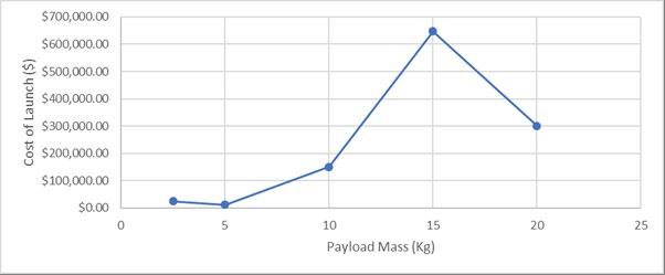
To determine the cost of the alternative method of acceleration, the muzzle velocity of the gun must be established. A computational program written by a research supervisor with support from the author was used to iteratively work backwards in time from the final orbital velocity. This program is can be requested via the author, and the process is described below. Due to the constraints of the coil gun system, the launches must occur in packets. This is because of the exponential growth in cost as packet size increases, see Figure 1
To simulate the path of the projectile, step back in set time frames (1s) and calculate the acceleration acting on the projectile for that period, to calculate the velocity before the step. To calculate the radius from the centre of gravity before the step, use the formula, �������� = ���������������� + 1 2 �������� �������� 2 , this produces a displacement for the time step, which is used to find the new radius.
The calculation of the effects of air resistance on the projectile is determined by using the velocity from the current step and the formula ���������������� = 1 2 ���������������� 2 ���������������� ��������. The formula solves for the force acting on the projectile (���������������� ), by taking the fluid density (��������), velocity (�������� ), drag coefficient (���������������� ) and area cross section (��������). Fluid density is sourced from the International Standard Atmosphere.
88 • Science Extension Journal Scientific Research in School Volume 4 Issue 1 2022
������������������������ ��������
���������������� 2 �������� .
The muzzle velocity of the projectile from the launch apparatus is used to calculate the kinetic energy required. The energy is converted to watt seconds, with the time required to achieve the muzzle velocity with the set acceleration (1000G | 9810m/s/s).
The watt seconds converted to kilowatt hours is used to estimate the energy cost based on local retail (0.4 cents/KwH) (Energy Australia)
Total Payloa d Mass (kg)
Traditional System Name
Launch Cost Coilgun Cost (2.5kg packs) Coilgun Cost (5kg packs) Coilgun Cost (10kg packs)
9 Vanguard $8,052,300 $88,039 $21,516 $135,653
122 Scout $13,639,600 $1,193,418 $291,662 $1,838,856
443 Pegasus XL $19,270,500 $4,333,475 $1,059,068 $6,677,157
540 Delta E $90,612,000 $5,282,340 $1,290,963 $8,139,199
632 Start $10,554,400 $6,182,294 $1,510,905 $9,525,877
820 Athena 1 $25,994,000 $8,021,331 $1,960,351 $12,359,524
1380 Taurus $28,152,000 $13,499,314 $3,299,128 $20,800,174
1500 Kosmos $12,000,000 $14,673,167 $3,586,009 $22,608,885
1500 Cosmos $18,600,000 $14,673,167 $3,586,009 $22,608,885
1850 Rockot $19,240,000 $18,096,906 $4,422,744 $27,884,291
2065 Athena 2 $34,279,000 $20,200,060 $4,936,739 $31,124,898
2177 Titan II $67,487,000 $21,295,656 $5,204,494 $32,813,028
2315 Delta 3910 $64,820,000 $22,645,588 $5,534,407 $34,893,046
3200 Long March 2C $32,000,000 $31,302,756 $7,650,152 $48,232,288
3630 Atlas Centaur $101,640,000 $35,509,064 $8,678,141 $54,713,502
4400 Dnepr $21,560,000 $43,041,290 $10,518,959 $66,319,396
5144 Delta II $78,703,200 $50,319,181 $12,297,619 $77,533,403
7000 Soyuz $53,200,000 $68,474,780 $16,734,707 $105,508,130
8292 Delta III $97,016,400 $81,113,268 $19,823,456 $124,981,916
8618 Atlas IIA $170,636,400 $84,302,236 $20,602,815 $129,895,580
9200 Long March 2E $70,840,000 $89,995,425 $21,994,187 $138,667,828
10060 H 2 $265,584,000 $98,408,040 $24,050,165 $151,630,255
10200 Ariane 44 $182,580,000 $99,777,536 $24,384,859 $153,740,418
13600 Long March 3B $85,680,000 $133,036,715 $32,513,146 $204,987,224
13740 Zenit 2 $60,456,000 $134,406,210 $32,847,840 $207,097,386
15875 Zenit 3SL $120,650,000 $155,291,018 $37,951,926 $239,277,366
17700 Titan Centaur $198,240,000 $173,143,371 $42,314,903 $266,784,842
17700 Titan IV $437,190,000 $173,143,371 $42,314,903 $266,784,842
18000 Ariane 5G $235,800,000 $176,078,005 $43,032,105 $271,306,619
18600 Saturn IB $321,780,000 $181,947,272 $44,466,508 $280,350,173
19760 Proton SL 13 $81,016,000 $193,294,521 $47,239,688 $297,834,378
22800 Falcon 9 $62,016,000 $223,032,139 $54,507,332 $343,655,051
27500 Shuttle $1,697,300,000 $269,008,063 $65,743,493 $414,496,224
63800 Falcon Heavy $89,958,000 $624,098,706 $152,524,904 $961,631,240
140000 Saturn V $728,000,000 $1,369,495,593 $334,694,147 $2,110,162,596
Science Extension Journal • 89 Scientific Research in School Volume 4 Issue 1 2022
Traditional
Table 1: Comparison of Traditional and Experimental Launch Methods of Equal Payload Sizes
Discussion
The results illustrate that while generally, the experimental method is more cost effective, the more modern traditional systems outperform the experimental method. As seen in figure 2 the Falcon Heavy (63800 kg Payload) outperforms all variants of the coilgun, however, the Saturn V (140000 kg Payload) only outperforms the coilgun in 2.5 kg and 10 kg packages. This suggests that this method may
be viable, as it is only beaten by much heavier rockets designed for longer voyages. The 10kg has a higher cross section, increasing the drag during the launch. However, both the 2.5kg and 5kg packs use the same cross section, allowing the 5kg packs to before better than the 2.5kg.

The outlier that is apparent in figure 2 is the Space Shuttle Program (27500 kg Payload), this is due to

90 • Science Extension Journal Scientific Research in School Volume 4 Issue 1 2022
Figure 2: Comparison of Traditional and Experimental Methods (Payload Size vs Cost)
Figure 3: Comparison of Traditional and Experimental Methods (Payload Size vs Cost) Zoom in
the high experimental efforts of the program and did not have technologies that are now available to us. Figure 3 shows a more refined view of the data, showing a greater comparison between the experimental method and traditional methods. The Falcon 9 (22800 kg Payload) is a common rocket used today, as seen in figure 3 the 5 kg variant is slightly more cost effective. However, these are estimations that do not include the addition of errors between launches. For this data to be of greater accuracy and value additional factors must be considered, such as maintenance, cost of the sabot, and potential costs due to excessive usage. The data is far from perfect, but still grants a relatively accurate representation of the costs of launching a projectile into LEO.
The data, in general, supports my hypothesis, however, the values in comparison to the modern day standards do not vary significantly.
Conclusion
The data illustrates that the usage of experimental coilgun designs to achieve Low Earth Orbit (LEO) is either less or not significantly more cost effective compared to traditional rocketry. The experimental method may become more viable due to the discovery of technology, however, I would suggest against investing our time into following these methods. This is because the value that would potentially be achieved within this context would be drastically less than if we invested the same value into traditional rocketry methods. The technology could be used for tools of destruction, therefore, there is still a potential use for this technology, however, would not have the clearest of ethics as utilised in my report.
Acknowledgements
I would like to acknowledge Dr Matthew Hill for his support as my supervisor and the author of the program I used to generate an appropriate muzzle velocity with a correlation to air resistance and gravitational acceleration.
References
Farr, R., Wilson, K., Young, P., Goossens, D., & Champion, N. (2018). Physics in focus. Year 12 (2nd ed.). Nelson, An Imprint Of Cengage Learning Australia.
Hou, C., Yang, Y., Yang, Y., Yang, K., Zhang, X., & Lu, J. (2020). Electromagnetic launch based method for cost efficient space debris removal. Open Astronomy, 29(1), 94 106. https://doi.org/10.1515/astro 2020 0016
Jones, H. (2018). The Recent Large Reduction in Space Launch Cost
Klyushnikov, V. Y. (2020). Dynamic Mass Accelerators From Past to Future. Aerospace Sphere Journal, 2, 62 71. https://doi.org/10.30981/2587 7992 2020 103 2 62 71
Markusic, T. (2010). SpaceX Propulsion Tom Markusic Space Exploration Technologies 46th AIAA/ASME/SAE/ASEE Joint Propulsion Conference https://kosmonauta.net/wp content/uploads/2010/08/images.spaceref.com_news_201 0_SpaceX_Propulsion.pdf
Marshall, R. A. (1981). Railgun Energy Stores and Systems. Utexas.edu. https://doi.org/PN_67
McMillan, E. M. (1945). The Synchrotron A Proposed High Energy Particle Accelerator. Physical Review, 68(5 6), 143 144. https://doi.org/10.1103/physrev.68.143
McNab, I. R. (2003). Launch to space with an electromagnetic railgun. IEEE Transactions on Magnetics, 39(1), 295 304. https://doi.org/10.1109/tmag.2002.805923 https://research.lifeboat.com/ieee.em.pdf
Mercado, M. (2019). Thermo Fluid System Level Modeling For The Crome And Crome X Ground Propellant System Using Generalized Fluid System Simulation Program https://scholarworks.utep.edu/cgi/viewcontent.cgi?article= 1118&context=open_etd
Niederstrasser, C. (2018). Small Launch Vehicles A 2018 State of the Industry Survey. Northrup Grumman Corporation.
Reddy, V. S. (2018). The SpaceX Effect. New Space, 6(2), 125 134. https://doi.org/10.1089/space.2017.0032
Reuter, C., & German Canadian Museum Of Applied History. (1998). The V2, the Russian and American rocket programm [sic]. German Canadian Museum Of Applied History.
SPACE SHUTTLE ASCENT Background. (n.d.). https://www.nasa.gov/pdf/466711main_AP_ST_ShuttleAs cent.pdf
Zabar, Z., Naot, Y., Birenbaum, L., Levi, E., & Joshi, P. N. (1989). Design and Power Conditioning for the Coil gun IEEE. https://www.ece.ucf.edu/seniordesign/sp2014su2014/g10/ research/other_sources/00022613.pdf
Zimmerman, A. (1966). EXPLORING IN AEROSPACE ROCKETRY LAUNCH VEHICLES https://ntrs.nasa.gov/api/citations/19680010821/download s/19680010821.pdf
Science Extension Journal • 91 Scientific Research in School Volume 4 Issue 1 2022
92 • Science Extension Journal Scientific Research in School Volume 4 Issue 1 2022
Rosco Jones
Barker College
Purpose: Through a comparison of first stage re use modes in the Falcon 9 launch vehicle a viability assessment of a “flyback” (Landing horizontally under the influence of aerodynamic forces) booster can be achieved.
Design: Data from the existing modes of launch demonstrated by the Falcon 9 were collected and analysed. A base set of assumptions about the Falcon 9’s performance were produced. Using assumptions produced a flyback mode of re use was designed and comparative evaluation was performed.
Findings: A flyback mode of re use was found to produce a reduction in inert mass relative to that of a retro propulsively landed booster, resulting in improved performance of re usable first stages.
Limitations: The experimentation was performed entirely theoretically utilizing an assumed data set. Real world properties of the Falcon 9 may differ greatly from that which was assumed. Practical validation of results produced are necessary for confirmation of validity.
Practical implications: Implementation of technologies which improve launch performance results decrease in cost of launch, increasing access to space.
Social implications: As a result of this cost reduction smaller groups will be capable of affording to launch their payloads. This will enable educational and scientific payloads which have no profit incentive a greater ability to launch.
Originality: Minimal research into Flyback boosters has been performed. Of the comparative research undertaken almost all has centred on the usage of theoretical modelling of all booster performance. This experiment instead utilizes data from real launches to increase validity.
Key words: Rockets, Re usable launch vehicles, Booster, Re usable booster, Retro propulsive landing, Flyback, Falcon 9
Glossary
Booster First stage of a rocket
Expendable Booster Booster that is not recovered
Re usable Booster Booster that is recovered and reused for future launches
Flyback Re usable booster that uses a plane like recovery method
Glideback Re usable booster that uses a glider like recovery method
Retro-propulsion landing Re usable booster the lands vertically in reverse to how it was launched
Payload Non vehicle mass being launched
Wet Mass Mass of a loaded vehicle
Dry Mass Mass of an unloaded vehicle
Literature Review
Launch costs are a primary limiting factor in humanities expansion into space (Chow, 2022). As
such many means of reducing costs are being explored. A commonly proposed means of achieving this is through re usable spacecraft (Jones, 2018). Improving the launch efficiency of re usable vehicles is the primary goal of this paper.
The implementation of a reusable system on a launch vehicle is inevitably to the detriment of its performance, relative to that of an expendable launch vehicle (R. Thompson, 2019). This is because re usable systems must include additional elements to enable the extended mission goal of re use. This is most notable in its effect on payload capacity, with the SpaceX’s Falcon 9 significantly reducing its payload capacity when reusing boosters in RTLS format (SpaceX, 2021). This has a substantial effect, being reduced from 12,605kg to 9,135kg (Schilling, 2009).
Despite the detriment to overall performance
Reusable Launch Vehicles have become the focus of the commercial launch market. Expensive components
Science Extension Journal • 93 Scientific Research in School Volume 4 Issue 1 2022
Did SpaceX get it wrong? A systematic evaluation of the potential of a flyback return mode to increase performance
form a disturbingly large portion of vehicle cost, with engines alone making up roughly 60% of all launch costs (Drenthe, Zandbergen, & Van Pelt, 2017). Components such as engines can be readily re used as refurbishment cost is minute relative to that of construction.
Expendable first stages are already well equipped to deal with the stresses of re entry. This is evidenced in their remarkably intact state (see Figure 1)

This is not the case with upper stages which tend to completely disintegrate after re entry due to atmospheric heating because of immense speeds (See Figure 2).

As such First stages will be the focus of this paper. For this paper two re use “modes” were chosen:
1. Main engine retro propulsion
2. Flyback utilizing plane like format
These were chosen as they are believed to be the most competitive forms of re use for vehicles with payloads 2,000 20,000kg. This is the most common lift range of vehicles currently on the market (Spaceflight101, 2017).

94 • Science Extension Journal Scientific Research in School Volume 4 Issue 1 2022
Figure 1: A Gemini fist stage being recovered from the ocean (Source: NASA, 1965)
Figure 3: Falcon 9 second stage debris in night sky (Source: Berger, 2021)
Figure 2: Falcon 9 re use mode flight paths (After SpaceX, 2019)
Retro-propulsion
Main engine retro propulsion utilizes the main engines of the first stage to provide oppositional thrust to the direction of movement, resulting in a decrease in momentum as shown in Figure 3. Main engine retro propulsion necessitates additional inert mass for the first stage of the launcher. This comes in the following forms:
Excess fuel
struts
strut support mechanisms
fins
Figure 4: Supersonic retro propulsion for mars rovers (Source: Mandalia and Braun, 2015)

SpaceX’s success in the field of Retro propulsive landings have become the majority focus of the Spaceflight industry, leading to competing concepts being largely ignored due to the “field tested” nature of retro propulsion. This becomes problematic as potentially superior design solutions have been abandoned. The flyback re use mode is a prime example of a competing system that has been under evaluated. Flybacks offer a range of unique advantages (Keith & Rothschild, n.d.) to the current launch market, with potential reductions in logistical costs and launch costs as well as their inherently safer design making them a compelling candidate.
Flyback
The Flyback re use mode utilizes aerodynamic forces to slow the vehicle, eventually enabling it to land much in the same way a plane does. To achieve this, it utilizes the following additional components:
Control systems
gear
Airbreathing engines (Glideback if not present, Flyback if present)
The mission of this paper is to estimate the ramifications of a flyback re use mode on the performance of a booster. The Falcon 9 was selected as a model for the comparison of these two models as it’s the only re usable booster to launch a payload to orbit. Both Flyback modes will be modelled.

The use of the Falcon 9
The Falcon 9 is a 2 stage, partially reusable space vehicle (See Figure 4). Its most notable feature is its re use of its first stage. It was selected for use in this research paper as a case study upon which the two re use modes can be compared. This is due to the expansive collection of data on its launches and its prevalence as the first ever reusable space vehicle to utilize retro propulsive landings. These factors all made it particularly attractive as a basis upon which flybacks can be fairly compared.
Several variants of the Falcon 9 exist. These are denoted by “Blocks”. Block 3 was selected as the ideal candidate as it has a publicly available data sheet on its characteristics (Espace and Exploration, 2017). This greatly increases experimental validity. This experiment will only utilize data from Block 3 launches. This is because there is a performance gap between variants.
Scientific Research Question
What effect will the implementation of a flyback system on a SpaceX Falcon 9 first stage in the place of a Retro propulsive landing system have of the cost per kilogram taken to orbit?
Scientific Hypothesis
That a flyback system will generate a smaller amount of excess weight relative to retro propulsion type
Science Extension Journal • 95 Scientific Research in School Volume 4 Issue 1 2022
1.
2. Landing
3. Landing
4. Grid
1. Wings 2.
3. Landing
4.
Figure 5: Falcon 9 Block 3 internal diagram (Source: Jenie, W. W. H. Suarjaya, & Poetro, 2019)
reusable vehicle and thus produce a greater payload capability.
Methodology
The following steps must be undertaken to enable a comparison of re use modes:
1. Data on Falcon 9 Block 3 was collected
2. Retro propulsion mode component weights were calculated
3. Retro propulsion component weights were subtracted to estimate expendable weight
4. Flyback mode was designed for Falcon 9 Block 3 fuselage
5. Flyback component weights were calculated for powered and unpowered modes
6. Flyback component weights were subtracted from total fuel mass of expendable booster for both flyback modes
7. Performances of all modes calculated
8. Analysis of launch performances was performed comparing payload mass capacity between each vehicle.
Modelling the Falcon 9 Grid Fins
The Falcon 9 utilizes a set of 4 grid fins to assist control during the descent phase of the flight. Grid fins are a commonly used form of control surface used in place of conventional planar fins for their high level of control at subsonic and supersonic speeds (See Figure 7). Whilst ideally these would remain in place for the flyback design their drag characteristics are far too great for efficient use and will be replaced.
Figure 7: Simulated wind tunnel testing of Callisto control surfaces (Source: DLR, 2018)

Grid fins are mounted towards the top of the Falcon 9’s first stage fuselage to provide self correcting drag when deployed, as well as generating a greater level of control due to their distance from the centre of mass (See Figure 8)
Figure 6: A 3D model of the Falcon 9's titanium grid fin (Source: Ross, 2022)

Figure 8: Falcon 9 with stowed titanium grid fins (Source: Henry, 2017)

The volume was of this model was found to be 44L when scaled appropriately. This was then used in conjunction with titanium’s accepted density of 4.5g/cm3. The weight of each Grid fin was thus found to be 198 kg, Bringing total weight of grid fins to 792kg.
Landing Legs
Landing Legs are support structures For the Falcon 9. They provide a wide base for the booster to prevent toppling and allow for inaccuracies in booster landing. Whilst large in size, as depicted in Figure 10, they are relatively light, weighing 600kg each (SpaceX, 2013).
96 • Science Extension Journal Scientific Research in School Volume 4 Issue 1 2022
Using a carbon fibre tubing calculator (Giordano, 2018) and assuming the average width to be 40cm, with tubing assumed to be 2cm thick and 12m long, weight of pistons is estimated to be 200kg.
A composite wrapped pressure vessel would also be used to store helium. This would be greater than 200kg, with an additional 100kg of fluid management systems (“Infinite Composites Pressure Vessels,” 2022). This brings the Landing legs and subsequent systems total weight to 4,400kg
Table 1: Falcon 9 Block 3 weight performance for various modes (After Schilling, 2022)
Recovery Method Payload to a 185km circular orbit Reduction in performance
No attempt at recovery
Ocean based drone ship recovery
Return to launch site
18,132kg (16,052 20,414kg, 95% confidence interval)
13,581kg (11,929 to 15393kg, 95% confidence interval)
11,410kg (10,057 12,763kg, 95% confidence interval) 37%
The Falcon 9’s second stage and fairings will remain constant regardless of the method of re use. This means we can treat the first stages potential change in momentum, or Δν, as the only point of difference between each result. Given we have the masses of each component as indicated in table 1 we are able to determine the fuel retained for each form of landing.

Table 2: Specification sheet for Falcon 9 Block 3 booster with re use structural mass (Espace and Exploration, 2017)
Stages Mass dry (kg) Mass wet (kg) Fuel Mass (kg)
1st stage 22,200 443,100 420,900
2nd stage 4,000 111,500 107,500
Fairing halves 4,450 4,450 0
Total 30,650 549,050 528400
This table is limited however as it is assuming the use of a re usable first stage. Using previously calculated structural weight adjustments it was adapted into Table 3:
Table 3: Specifications sheet for expendable Falcon 9 first stage (After Espace and Exploration, 2017)
Stages Mass dry (kg) Mass wet (kg) Fuel Mass (kg)
1st stage 17,008 437,908 420,900
2nd stage 4,000 111,500 107,500
Excess Fuel
Using Schilling’s calculator and values attained, we can determine the relative performance of each mode of re use for currently existing Falcon 9 variants, finding their maximum payload to given orbits. With the calculator, it was possible to produce the following table for the Falcon 9 block 3:
Fairing halves 4,450 4,450 0
Total 25,458 543,858 528400
We are now capable of determining the Δν of each stage of the rocket. This can be achieved using Equation 1.

Science Extension Journal • 97 Scientific Research in School Volume 4 Issue 1 2022
Figure 9: Falcon 9 landing leg in comparison to man (Source: Jurvetson, 2017)
Figure 10: Falcon 9 with legs fully deployed on drone ship (Source: Jeven, 2017)
N/A
25%
For all sea level engines, it is assumed there will be a constant instantaneous thrust of 6,444 Kn. Values from the tables were subbed into the equation to find the Δν of the first stage for both re use modes.
The second stage was found to have a Δν of 11,148m/s. This does not include the fairing. Fairing separation was timed from the ignition of the second stage over 3 launches of the Falcon 9 Block 3 and was consistently 20 seconds after ignition. Δν of the second stage before separation was found to be 795m/s, and after; 9,822m/s. This brings the second stages total Δν to 10,617m/s.
The results of these equations in shown in Table 4.
Table 4: Retro propulsion vs Expendable performance (After Espace and Exploration, 2017)
Mode Δν Standalone (m/s)
with upper stage (m/s)
Retro propulsion 8,083 3,814
Expendable 8,770 4014
Second stage 11,148 10,617
The retro propulsion re use mode has a total Δν capacity of 14,431m/s. The expendable booster has a capacity of 14,631m/s. This means that there is a 1.5% disparity between the total Δν capacity of the two rocket formats. This is a near negligible margin.
As such it can be determined that the loss of 25% of payload capacity is almost entirely due to the conservation of fuel for re use in the drone ship landing scenario. Due to time requirements properly calculated estimates were unable to be made and thus It was consequentially decided that a conservative 20% excess fuel margin for the would be employed for use in this research paper. This brings the total excess fuel weight to 84,180kg for a drone ship landing. It is assumed that 40% or 33,672kg of this fuel mass is reserved for the entry burn.
For a RTLS mission this mass fraction is even greater, with 37% of payload capacity being lost. As such a conservative 30% excess fuel margin was employed. This leads to an excess fuel weight of 126,270kg for RTLS missions.
Modelling of a flyback system
The main comparative aspect of these is to gain a weight estimate for each component as it will have the
most influence on overall payload performance. To estimate the masses of each component a variety of methods must be utilized. Fortunately, as flybacks utilize common components with aircraft due to them performing a similar action. This enables accurate adjustments of fuselage weight to accommodate additional structures to support plane like loads.
new components are
Fuselage weight
weight
gear
engine and supporting systems
Fuselage weight
There is a high likelihood alteration to the fuselage will be necessary to accommodate the aerodynamic stresses during flight. This is however hard to calculate as SpaceX have already included stringers and ribs into their design (see Figure 11).
The exact weight of struts needed to accommodate for additional loads would require specific data on the Falcon 9 fuselage which is unavailable. To account for this additional mass a further 3,500kg of structural mass will be added.

Wing weight
The primary additional weight of the flyback booster design will be its wings, and as such needs to be calculated carefully. The Falcon 9 has a side area of roughly 150m2. The boosters’ wings are unable to deviate from the side profile of the Falcon 9 to any notable extent as in doing so they will incur immense structural stresses during re entry as they would no longer be shielded by the fuselage itself. The wing mounting location will further limit the wing in size
98 • Science Extension Journal Scientific Research in School Volume 4 Issue 1 2022 ���������������� = ∫ |�������� (�������� )| �������� (��������) ������������������������ 1 ��������0 (1)
Δν
The
1.
2. Wing
3. Canards 4. Landing
5. Optional
Figure 11: Internal view of SpaceX ring structure (Source: Goff, 2006)
however, as for ideal flight the wing will need to be mounted near the centre of gravity so as to ensure the centre of lift remains near it (see Figure 12).

Figure 12: A selection of wing formats (Source: Ravi, 2020)
As a result of this it was decided a conventional plane design would not be optimal for these restrictions. Below are several proposed options:
It was decided a lifting canard design without a vertical stabilizer would be optimal as there would be four canards spaced evenly around the front, granting both axis of control. This can be seen in Figure 13. The implementation of this design is showcased in Figure 14

Figure 14: from left to right: Expendable mode, Retro propulsion mode, Flyback mode (After: SpaceX, 2020)

Using Figure 13 in combination with basic area equations, it is estimated that the flyback booster will have a total wing area of 120m2. Using Figure 15 17 we can determine that the plane’s wing is expected to be 15,849kg in total.
Figure 13: Diagram of Canard controls (Source: Osheku, 2018)
Figure 15: Wing weights vs area of Plane and bird wings (Source: Liu, 2006)

Science Extension Journal • 99 Scientific Research in School Volume 4 Issue 1 2022
This is subject to inaccuracy as the booster will still be required to accommodate for the hinging of the wings on the aircraft. As such the mass estimate was increased by 20% to accommodate for additional structural mass, bringing total wing weight to 19,018kg.
Canard weight
The Flyback mode Falcon 9 will utilize conventional planar Canards similar to those in Figure 17 as opposed to the grid fins previously utilized by the Retro repulsively landing Falcon 9 variant. This reduces drag, extending the boosters range upon re entry and for the duration of flight.
Canard dimensions were determined in accordance with recommendations from the NASA technical memorandum. As such Canards were determined to be 1/10th of each wings area. Canard dimensions are as depicted in Figure 17.
The weight of the Canard was then estimated through the same process as the original fold out design. This gives us an estimated weight for each Canard of 316kg, Bringing the total weight of canards to 1,265kg.
Engine weight
The CFM56 7 weighs 1,940kg. For a sustained flight speed of 250m/s the rocket will thus require 2,800kg of additional fuel (Almahmood, Bradley, Soret, 2022). This brings total additional engine weight to 4,740kg.
Landing gear weight
With conventional planes, it can be assumed that landing gear weight will be 2.5 5% of the maximum take off weight. We will instead use the dry mass of the booster as it will be the only weight applicable during touchdown. We can estimate landing gear weight to be 1019kg for the Glideback booster and 1,138kg for the Flyback booster.
Re-entry Burn
The re entry burn for each booster was determined to cost an additional 33,672kg. As the Flyback and Glideback boosters both require a re entry burn this will be added to their inert weight.
Results
Total retro propulsion additional mass
The total additional weight necessary for the falcon 9 to perform a retro propulsive landing is 106,380 kg, assuming it can land down range. This is then increased by 42,090 kg when a return manoeuvre is employed. The final inert mass of a RTLS mission is 148,470 kg.
Total Flyback additional mass

The total mass of the flyback booster

100 • Science Extension Journal Scientific Research in School Volume 4 Issue 1 2022
Figure 16: Wing weight and span of Plane and Bird wings. (Source: Liu, 2006)
Figure 17: Trapezoidal shape of Canard
Finalized first stage properties
The final weight of components for the unpowered Flyback booster is 57,455kg in total. With the addition of engines and reserve fuel it becomes 62,195kg. These properties combined with those in Tables 2 and 3 were combined into Table 5 for comparison.
Table 5: Finalized flyback booster properties
Booster Inert Mass (kg) Contributed Δν (m/s)
Expendable 17,008 3,921
Glideback 74,463 2,923 Flyback 79,203 2,855
Drone Ship retro propulsion 106,380 2,496
Return to launch site 148,470 2,019
Payloads to orbit
Using the open source calculator “Launcher” Maximum payloads to orbits between 250 4000km were graphed for each variant. This is shown in table 6. This indicates the expendable booster has significantly greater weight to orbit performance than that of reusable modes. The flyback modes are significantly smaller than that of the payload weight.

Discussion
This investigation’s goal was to assess the ability for a flyback system to reduce excess inert weight. Through the usage of the SpaceX Falcon 9 rocket as a framework for a re usable booster we were able to accurately compare re use modes. This experiment demonstrated a reduction in additional inert weight for Flyback boosters relative to that of the retro propulsion type re usable boosters, resulting in an increase in payload. This is in support of the hypothesis.
Figure
Weight
altitude
This experiment was carried out in an effort to supplement the work of Martin Sippel, who has carried out extensive evaluations of re usable boosters. Sippel’s work has almost always centred upon designing rockets from the ground up, creating extremely accurate Figures which can then be utilized in the comparison of re use modes (Bussler & Sippel, n.d.). This research paper centred upon using the Falcon 9 as a case study for the re use of rockets, taking the existing design of the Falcon 9’s first stage as well as its expendable variant and constructing a theoretical model of a Flyback stage from this foundation. This sacrifices the precision favoured by Sippel’s experimentation but enables an increase in experimental accuracy as a flight proven re usable booster is being utilized as a point of comparison. This was done as the resources to undertake the extensive process of developing a re usable booster from the ground up and modelling its use were not available.
Science Extension Journal • 101 Scientific Research in School Volume 4 Issue 1 2022
18:
vs
of Falcon 9 variants
Another point of difference this paper wished to explore was the difference in payload capacity present between each vehicle. This was seen as a valuable contribution as a large portion of flyback booster design research has had a greater focus on the economics of booster re use rather than actual performance metrics (Stappert, Wilken, Bussler, & Sippel, n.d.). As a result of this there is little understanding potential advantages posed by the use of a flyback system to enhance or denigrate the performance of a vehicle. This paper aimed to provide the answer to this issue.
This experiment demonstrated the ability for aerodynamic forces to mitigate and re direct the energy imparted on a rocket during re entry with less of a toll on performance than that of retro propulsion under the power of a rockets main engines. The findings of this study indicate a strong potential for the usage of a reusable Flyback systems in the place of retro propulsion mode reusable vehicles. Their improvement on payload mass makes them an attractive candidate in the space launch market. Flyback type re usable launch vehicles require further investigation and research as their potential to mitigate the cost of space travel is only increasing with each iteration of research.
The approach taken in this research paper allows for continual improvement as data collected retrospectively to be easily substituted in, improving the accuracy and reliability of results derived. There is also constant room for improvement in the component weight estimates, particularly that of wings, excess fuel and fuselage. These components should be more precisely calculated in future experimentation to provide a more reliable result. Inaccuracies in the measurement of components are a large component of experimental error present. Through the use of a case study with more publicly known specifications accuracy may be improved. This was a large source of error as the data available could not be verified.
The data was shown to be very uniform as seen in Figure 18. This is believed to be because of limitations in tools utilized. The “Launcher” calculator was unfortunately the only available means of determining maximum payload masses. This software, whilst useful, is incredibly inaccurate in its predictions, utilizing a linear scale to predict maximum payloads to each orbit. This is detrimental to the experiment as the relationship between maximum payload and orbital height is non linear, and thus the calculator was producing incorrect results. As such table 6 should be considered a visual representation of data presented in
table 5 rather than legitimate statistics. Whilst it would have been preferable to utilize Schilling’s calculator to perform a similar function this was not possible due to the calculator’s interface preventing the insertion of other vehicles for consideration.
Conclusion
This paper intended to establish a performance estimate for the payloads of re usable variations of the Falcon 9 to various orbits. In this paper there was a demonstrated reduction in inert weight due to the implementation of a Flyback system. Flyback systems were shown to outperform retro propulsive type re usable boosters in terms of payload for all orbits. This is through the use of aerodynamic forces to slow and direct descent in the place of fuel intensive propulsive landings. Whilst research has shown potential economic incentives for the adoption of Flyback systems this experiment has demonstrated an increase in payload performance. Though research is limited in accuracy, error can be greatly reduced through utilization of new data and more comprehensive mass estimates. It should be stressed that further research must be carried out validate results.
Acknowledgments
This paper would not have been possible if it were not for the immense support of the following people. Their contributions and sincerely appreciated
Dr Mathew Hill for providing experience and advice in the production of this paper. Dr Cameron Dearn for assistance with physics related components of this paper. Thomas Leach for his immense help with developing potential mathematical solutions to this paper and all the remaining Science Extension staff for their understanding and assistance throughout my project.
References
Chow, D. (2022, April 8). How falling launch costs are fueling the thriving space industry. Retrieved June 21, 2022, from NBC News website: https://www.nbcnews.com/science/space/space launch costs growing business industry rcna23488
Jones, H. (2018). The Recent Large Reduction in Space Launch Cost. Tdl.org. https://doi.org/ICES_2018_81
Launch Vehicle Performance Calculator. (2022). Retrieved May 15, 2022, from Silverbirdastronautics.com website: http://www.silverbirdastronautics.com/cgi
102 • Science Extension Journal Scientific Research in School Volume 4 Issue 1 2022
SpaceX. (2022). SpaceX. Retrieved May 14, 2022, from SpaceX website: https://www.spacex.com/ Giordano, R. (2018). Drone Tubing Calculator. Retrieved May 14, 2022, from Design215 website: https://design215.com/dcal/toolbox/tubing calculator
Infinite Composites Pressure Vessels. (2022). Retrieved May 14, 2022, from Infinitecomposites.com website: https://www.infinitecomposites.com/infinite composite pressure vessels
bin/LVPcalc.pl
“Fiche Technique: Falcon 9” [Technical data sheet: Falcon 9]. Espace and exploration (in French). No.39 May 2017. Pp. 36 37. Retrieved May 18, 2022 from
Jones, H. (2018). The Recent Large Reduction in Space Launch Cost. Retrieved from https://ttu ir.tdl.org/bitstream/handle/2346/74082/ICES_2018_81.pdf
Alcantarilla, A. (2022, March 18). SpaceX sets new booster reuse record on Starlink mission. Retrieved June 7, 2022, from NASASpaceFlight.com website: https://www.nasaspaceflight.com/2022/03/spacex booster reuse record
starlink/#:~:text=MVac%20ignition%20occurred%20at%2 0around,separated%20about%2020%20seconds%20later.& text=Falcon%209’s%20payload%20fairing%20is,down%2 0to%20the%20Atlantic%20Ocean.
Electron | Rocket Lab. (2022). Retrieved June 18, 2022, from Rocket Lab website: https://www.rocketlabusa.com/launch/electron/ NASA Solid Rocket Boosters. (2022). Retrieved June 18, 2022, from Nasa.gov website: https://www.nasa.gov/returntoflight/system/system_SRB_p rt.htm
Lone, Mohammad & Saeed, Tariq & Graham, Will & Babinsky, Holger & Jarrett, Jerome & Hall, Cesare & Seffen, Keith & Eastwood, Jeremy. (2009). Conceptual Design for a Laminar Flying Wing Aircraft. 10.2514/6.2009 3616.
Berger, E. (2021, March 26). A Falcon 9 rocket making an uncontrolled re entry looked like an alien armada. Retrieved June 20, 2022, from Ars Technica website: https://arstechnica.com/science/2021/03/a falcon 9 rockets second stage just burnt up over seattle/ Stappert, S., Wilken, J., Bussler, L., & Sippel, M. (n.d.). A Systematic Comparison of Reusable First Stage Return Options. Retrieved from https://elib.dlr.de/128623/1/EUCASS2019_AKIRA_438_fi nal.pdf
Keith, E., & Rothschild, W. (n.d.). Propulsion system advances that enable liquid fly back booster (LFBB) Retrieved from https://core.ac.uk/download/pdf/10474026.pdf
Jenie, Y. I., W. W. H. Suarjaya, & Poetro, R. E. (2019). Falcon 9 Rocket Launch Modeling and Simulation with Thrust Vectoring Control and Scheduling. Retrieved June
20, 2022, from undefined website: https://www.semanticscholar.org/paper/Falcon 9 Rocket Launch Modeling and Simulation with Jenie Suarjaya/2573a201f08cc1d57b2b0dd3b6616f23688131e5
Thingiverse.com. (2022). Hypersonic Grid Fin SpaceX Falcon 9 608 Bearing Edit (Flap and Pitch) by caross. Retrieved June 20, 2022, from @thingiverse website: https://www.thingiverse.com/thing:5279023/files
Steve Jurvetson. (2022, June 20). Retrieved June 20, 2022, from Flickr website: https://www.flickr.com/photos/jurvetson/13928869164 Drenthe, N., Zandbergen, B., & Van Pelt, M. (2017). Cost Estimating of Commercial Smallsat Launch Vehicles https://doi.org/10.13009/EUCASS2017 286
Goff, J. (2021). SpaceX COMSTAC Briefing | Selenian Boondocks. Retrieved June 20, 2022, from Selenianboondocks.com website: https://selenianboondocks.com/2006/10/spacex comstac briefing/
Ravi, V. (2020, November). Design of a Commercial Narrow Body Aircraft. Retrieved June 20, 2022, from ResearchGate website: https://www.researchgate.net/publication/349311912_Desi gn_of_a_Commercial_Narrow_Body_Aircraft Osheku, C. (2018). Retrieved June 20, 2022, from Intechopen.com website: https://www.intechopen.com/chapters/64567
Almahmood, Bradley, Soret (2022). Retrieved June 21, 2022, from CFM International website: https://www.cfmaeroengines.com/press articles/cfm56 7 an in depth look at the new industry leader/
Bussler, L., & Sippel, M. (n.d.). Comparison of Return Options for Reusable First Stages. Retrieved from https://elib.dlr.de/112470/1/Comparison_Of_Return_Optio ns_L.Bussler_M.Sippel.pdf
Stappert, S., Wilken, J., Bussler, L., & Sippel, M. (n.d.). A Systematic Comparison of Reusable First Stage Return Options. Retrieved from https://elib.dlr.de/128623/1/EUCASS2019_AKIRA_438_fi nal.pdf
Spaceflight101. (2017, December 31). Retrieved June 21, 2022, from Spaceflight101.com website: https://spaceflight101.com/2017 space launch statistics/
Science Extension Journal • 103 Scientific Research in School Volume 4 Issue 1 2022
104 • Science Extension Journal Scientific Research in School Volume 4 Issue 1 2022
The effect of the curvature of a swimming paddle on the propulsion force
Jessica Hargreaves Barker CollegePurpose: This paper aims to investigate the effect of the curvature of a swimming paddle on the fluid resistance and therefore propulsion force. Its purpose is to understand the optimal curvature for the highest propulsion force to allow for optimal muscle and technical development in training.
Design/methodology/approach: Swimming paddles of four different curvatures were attached via a bespoke apparatus consisting of a cable pulley system and secured before a pool swimming jet. The tensile force on the cable was measured for each manufactured swimming paddle.
Findings: This investigation found that the propulsion force increased until 20° when decreased after, producing a lower reading at 30° curvature. The implication of this data is that a paddle of approximately 20° curvature has the optimal propulsion force compared to angles above and below it.
Research Limitations/implications: An increase in curvatures tested would be an improvement of this investigation. Especially curvatures between 10° and 30° as the data implies that the optimal propulsion force is between these values.
Practical implications: The inconsistent flow from the jet caused the paddle to move back and forth, in turn causing the force on the luggage scale to fluctuate, potentially causing inconsistent results.
Social implications: This information allows for the swimming community to understand the most effect paddle to produce allowing them to be accessible and affordable to all.
Originality/value: While various elements of swimmers' hand position and spread have been investigated, to the author’s knowledge, research surrounding the effect of curvature of swimming paddles on propulsion force has not been published in any form

Keywords: Swimming paddles, Muscle growth, Propulsion force, Training, Fluid resistance
Paper Type: Research paper
Literature Review
Elite swimmers often include sets in their trainings involving the use of swimming paddles which requires an athlete strapping a plastic paddle to their hand (Ogita, 1999) (See Figure 1). The purpose of the paddles is to increase the resistance of the hands as they move through the water, in turn strengthening the swimmers’ arm, shoulder and back muscles. Therefore, it is desirable to maximize fluid resistance through water for a given surface area of paddle (of similar size to a human hand).
As for all sports, there has been extensive research into the mechanics of a swimmers’ stroke where they pull their hand and arm backwards through the water to propel them forwards (Tsunokawa, 2019; Houwelingen, 2017). Due to the need to maximize pulling force, a number of these studies focus on hand position and finger spread to optimize the force produced by the stroke.
Sidelnik and Young (2006) produced a study that experimentally simulated the dynamics of the freestyle stroke in the pull down phase by measuring
the propulsive force created by two models of human hands: one with fingers held together and the other held with fingers spread at 10∘. It was determined with 95% confidence that a finger spread of 10∘ creates more stroke force than a fingers together configuration across all pitch angles tested. This is due to the turbulence created between the fingers, in turn allowing for a larger propulsion force (Sidelnik and Young, 2006; Marinho, 2020; Vilas Boas, 2015).
Science Extension Journal • 105 Scientific Research in School Volume 4 Issue 1 2022
Figure 1: Photograph of man swimming with plastic paddles (Source: Smith, 2020)
Some experiments investigating both finger and thumb spread (Vilas Boas, 2015) shown in Figure 2.
for the combination of thumbs and fingers that are either separated or together (Vilas Boas, 2015).
The kinematic characteristics of the hand during a free style stroke were investigated through computer simulation and recording devices (Gouroulis, Aggeloussis, Vezos, Antonoiu & Mavromatis, 2008). The hand orientation for optimal angles was found to change as the hand progressed through the stroke. It was determined that the larger the hand the more force produced, and that the angle that produces the optimal force is perpendicular (90°) to the direction the body in the water is moving, however the position of the hand with respect to the body also influences the force created to propel forwards through the water. Another investigation modelled all the orientations of the hand and the fingers as shown in Figure 3 and 4 which revealed the propulsion force


Figure 4: Hand orientation (Source: Vilas Boas, 2015)
Other studies have focused on the use of paddles and their effect on producing the optimal force. Studies have shown that the larger the surface area of the paddles, the more resistance the paddle will have (Crocker et al., 2018, Hubb, 1991). The results from this study suggest that an optimal hand paddle size for proficient, adult swimmers is 210 358 cm2. The greater the surface area the more resistance and force that will need to be simulated to pull through the water. Therefore, the surface area of 210 358 cm2 for an average capable swimmer creates the optimal propulsion force whilst maintaining appropriate force and resistance on the swimmer’s body. It was also found that compared to free swimming, paddle
Figure 3: Results of different hand orientations (Source: Vilas Boas, 2015)
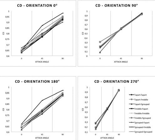
106 • Science Extension Journal Scientific Research in School Volume 4 Issue 1 2022
Figure 2: Hand models used in investigation of fingers and thumb spread (Source: Vilas Boas, 2015)
Figure 5: For both swimming free and paddle swimming, the data is given as mean (SD) of all measurements (N =45) on all subjects. The paddle and free swimming scores were tested for differences using a two tailed Student’s r test for paired comparison

(Source: Hubb, 1991)
swimming increases your work per stroke (Minetti, 2021; Hubb, 1991) as shown in Figure 5.
The optimal shape of paddles can be drawn from a study that focus of the fluid mechanics of the paddle wheel (Hildebrandt, 2020, Peterson, 2001). The study found that cylindrical paddles created a larger propulsion force compared to cubic paddles with the same surface area.
However only certain areas of this topic have been investigated such as the shape of the paddle, size and other factors that have been acknowledged and incorporated into the deeper understanding of this topic, and therefore it is important for this investigation to consider optimization of paddles for a given surface area and in turn making the independent variable of this experiment the concave curvature of the paddle. This gap in the literature relating to optimal paddle curvatures was the motivation behind this investigation.
Scientific Research Question
What is the optimal curvature of a swim paddle, to allow for maximum propulsion force?
Scientific Hypothesis
It is predicted that the force exerted by the swim paddle will increase as the angle of the curvature increase, until a certain point, then the force will begin to decrease.
Methodology Apparatus
The apparatus was invented during the course of this investigation for the sole purpose of testing the force
of water pushing against swimming paddles. The core of the apparatus was constructed out of two pieces of wood, drilled together at right angles, one piece horizontal and the other vertical, as shown in Figure 6. Two large hooks were screwed next to each other at the top of the vertical piece of wood to hold the luggage scales. Handheld luggage scales were used as when a force pulls them down they give a reading of a mass, which can be converted to force, using the formula F=ma. A small pulley was attached near the bottom of the vertical piece of wood, making sure it was above the water level. A narrow 25cm long piece of dowel was attached to the paddles on one side to increase the stability when testing. The other side of the dowel was attached to the string that went through the pulley and attached to luggage scales
Paddles
The four paddles were made from four different colored acrylic materials. Each sheet of acrylic was cut in a laser cutter with the 26x15cm oval being cut out of each one. They were all cut the same size to keep surface area constant. Once they were cut, they were placed in the oven at 200 degrees Celsius for 20 minutes to soften. While they were in the oven, four identical pieces of aluminum sheets were curved to four different curvatures (Figure 7), the angles were measured from the tangent of the top of the curve as shown in Figure 8. The angles included were 0° (flat piece of acrylic), 10°, 20°, 30°. Once the acrylic had softened, the acrylic was laid on the different curvatures as shown in Figure 7. After 20 minutes, once cool, it retained its curvature, and the final product is shown in Figure 9.
Science Extension Journal • 107 Scientific Research in School Volume 4 Issue 1 2022


108 • Science Extension Journal Scientific Research in School Volume 4 Issue 1 2022 Figure 7: Paddle production of curvatures 10° (green), 20°(orange) and 30°(yellow) Figure 8: method to form accurate curvature Figure 9: All four paddles made Figure 6: Experimental Setup
Experimentation
The experimentation process began by attaching the first paddle (0°) to the wooden dowel of the apparatus by tightly screwing the two together, as shown in Figure 6 and Figure 10. The dowel was then connected to the 1m long string that ran through the pulley and attached to the bottom luggage scale. The apparatus was set up on the edge of the pool with the vertical piece of wood directly above the mouth of the jet. Before lowering the paddle into the water, the luggage scale was zeroed, then the paddle was lowered into the water.
The force produced by the jet against the paddle caused a downwards force on the luggage scale, providing a mass reading (g). Since Force is proportional to mass, by the equation F=ma, as the mass increased, the force also did. Once a fixed mass was measured, the data was written down. This reading in grams was divided my 1000 to give kg, then times by 9.8 (acceleration due to gravity) to produce a force result.
The paddle was then taken out of the water to then zero the scale again. The experiment was repeated for 2 more trials for the 0° angled paddle, then that paddle was unscrewed from the dowel and the 10° paddle was attached. This was to keep the dowel and the string length constant for everything. The same process was completed for the 10°, 20° and 30° angled curvatures, therefore collecting three trials for each set of curvatures.
Results
Table 1 shows the results for each trial and the average force of the water pushing on each curvature of paddle. The results are then presented in graphical form in Figure 11.
Table 1: The force in Newtons pushing against each of the paddles according to their curvature.
Curv ature (°)
Figure 10: Fully constructed apparatus outside of the water with 0° paddle attached
Mean Force (N)Trial 1 Trial 2 Trial 3
Mass on scale (g) Mean Mass (g)
0 164 189 145 166 1.6268
10 140 168 201 169 1.6562 20 212 235 293 246 2.4108 30 190 167 207 188 1.8424
Paddle Curvature vs Propulsion Force
2.5
1.5
2
1
0.5
pushing against each of the paddles (N) Paddle Curvature (°)
3 0 10 20 30 40
0
Figure 11: Graph showing the relationship between the paddle curvature and the average propulsion force
While completing the experiment there were a number of qualitative observations about the behaviour of the paddles which assisted in the interpretation of the results. These are reported in Table 2.

Science Extension Journal • 109 Scientific Research in School Volume 4 Issue 1 2022
Force
Table 2: Qualitative Observations of the paddles positioning in the water and effect the water flow against it had, for each curvature
Paddle Curvature (°)

Observations
0 fell below the water flow line when unassisted was flimsy and unstable
10 on some attempts fell below the water flow line when unassisted was quite unstable, moved around
Held its position against the force of the water
Stayed sturdy and movement was limited
Held its position against the force of the water
Stayed sturdy and movement was limited
is able to be held throughout the pulling motion of the swimming stroke. This inversely proportional relationship means that the correct balance of both will result in the optimal propulsion force. The paddle curvature of 20° produces the optimal propulsion force as it’s amount of curvature effectively holds water whilst maintaining a large frontal surface area. As observed in Table 1, there is a lot of variation in the raw data used to make the averages. Whilst 20° is clearly higher than the others for all three trials, there is a lot of fluctuation amongst the others suggesting a lack of reliability in single tests. Therefore, three trials allowed the average of the trials to be used as a better representation of the data.
Discussion
The research question was to investigate what the optimal curvature of a swim paddle was, to allow for maximum propulsion force. The data produced through experimentation is shown in Table 1 and Figure 11. The relationship between the paddle curvature and the propulsion force in Figure 11 shows a minimal increase between 0° and 10° of only 0.0294N (1.6268N 1.6562N). Between 10° and 20° the propulsion force increases at a higher rate from 1.6562N to 2.4108N. It then began to decrease between 20° and 30°, with the paddle curvature of 30° having a propulsion force of 1.8424N. The results supported the hypothesis that the force exerted by the swim paddle will increase as the angle of the curvature increases, until a certain point, then the force will begin to decrease. This is evident in the graph in Figure 11, as there is an increase in force until 20° then it begins to decrease. Therefore, the certain point in which the force is maximized at for this experiment, is a curvature of 20°.
The conclusion drawn from these results is that the optimal curvature for a swimming paddle lies between 10° and 30°, evident in the results that show a peak between the two curvatures. This is due to the combination of curvature and surface area, which are both factors that influence the amount of water that can be held in a paddle. As a paddles curvature increases its frontal surface area decreases as shown in Figure 12. Frontal surface area is important as it allows for a larger amount of water to be pulled through when propelling through the water. Curvature is also important in making sure the water
Figure 12: Different curvatures producing different frontal surface areas with same sized paddle
While conducting the experiment, observations (in figure 15) highlighted the positioning of each paddle and how they reacted to the force of the water against it as shown in figure Curvature angles of 0° and 10°, when placed in the direct flow of the water, sunk below the flow as shown in Figure 13, causing the water to not directly contact the paddle. This was caused by the inability to hold water in the paddle, which is important for swim paddles as they must hold as much water as possible to then maximize the pull through the water. These two curvatures were also unstable and did not hold their position in the water, reiterating that the lower the curvature the less water that is able to be held in the paddle, in turn minimizing the stability of the paddle. Due to the instability of these paddles, when testing they had to be lightly held up to make sure that the water flow was directly hitting the paddle. They were held directly up with a piece of string around the wooden dowel, only being pulled in the upwards direction, not away or towards the apparatus to minimize the effect on the results.
110 • Science Extension Journal Scientific Research in School Volume 4 Issue 1 2022
20
30
As the curvatures increased the stability in the water increased as both the 20° and 30° paddles were able to stay stationary while being in the direct line of the water flow. This supports the concept that higher curvatures have the ability to hold water better, which is desirable when wanting to find a curvature that gives the optimal propulsion force.
The methodology of this investigation had limitations that restricted the overall outcome and results of the experiment. The amount of curvature angles measured and tested was limited to four in this investigation, reducing the overall knowledge of the relationship between the curvature of swim paddles and propulsion force. The limited number of curvatures made it hard to understand the trend, and other information relating to this experiment. This could be improved by including curvatures at 1 2 degree increments between 10 and 30° to gain a better understanding of the relationship.
Only three trials for each paddle were conducted throughout the experiment. This small sample size could misrepresent the correct and valid data. This could be improved by adding further trials in to remove outliers and gain valid and reliable data. The raw data received from this experiment varied a lot, making averages even more important as all of the raw data was so different.
Another limitation was the inconsistent flow of the water. The pool jet used in this investigation was dependent on the amount of water in the pool. For example, initial pre tests were conducted when the water levels were low, resulting in the water flow
being inconsistent and unreliable as it was causing the paddles to move back and forth, which produced unreliable results. The experiment was repeated, and final results obtained when the water levels were high again, which reduced the inconsistent flow, however it was still not flowing at a completely constant rate. To improve this, the experiment could be conducted in a flow tank or against a jet that produced a constant flow rate.
Another limitation of the experiment was that the paddles with curvatures of 0° and 10° had to be held up by a piece of string which may have affected the results for those two curvatures. This could be improved by doing this to all four of the curvatures to make the assistance constant throughout the entire experiment. Conducting the experiment in a flow tank may also address this limitation.
While a constant stream of water colliding with the paddle was an effective substitute for force output from a moving paddle, another expansion from this experiment could be investigating the curvature by pulling the paddle through the water using a weight and pulley system. This would simulate the exact movement of a paddle when it is being used by a swimmer.
Future projects relating to this investigation could include experimentation of the curvatures between 10° and 30° in smaller increments to find a more accurate value for the optimal curvature for a swimming paddle.

Science Extension Journal • 111 Scientific Research in School Volume 4 Issue 1 2022
Figure 13: Paddle sinking below the water flow
Conclusion
In conclusion the experimental data supported the hypothesis that the force exerted by the swim paddle will increase as the angle of the curvature increase, until a certain point, then the force will begin to decrease. The data showed that the optimal curvature of a swimming paddle was approximately 20 for maximum propulsion. This was found through experimentation using a pulley based apparatus to measure the force exerted on the paddle when in direct contact with water flow. While there was a clear maximum around 20°, further experimentation could increase the precision and reliability of the result including a greater variety of paddle curvatures, a higher volume of testing, and testing using various alternative apparatus.
Acknowledgments
I would like to thank Dr Matthew Hill for encouraging me to dive deeper into my research and explore an area of real interest to me. Thank you for regular conversations about the science process and troubleshooting ideas about the apparatus.
I would also like to thank Mr Tim Grimes (D & T teacher, Barker College) for assisting and guiding me through the design and production process of creating my four acrylic paddles that were used in the experimentation component of this investigation.
References
220 Triathlon. (n.d.). Swimming with paddles: a training session to develop power. [online] Available at: https://www.220triathlon.com/training/swim training/swimming with paddles a training session to develop power/ [Accessed 20 Jun. 2022].
Barbosa, A.C., Castro, F.D.S., Dopsaj, M., Cunha, S.A. and Júnior, O.A. (2013). Acute responses of biomechanical parameters to different sizes of hand paddles in front crawl stroke. Journal of Sports Sciences, 31(9), pp.1015 1023. doi:10.1080/02640414.2012.762597
Crocker, G.H., Moon, J.F., Nessler, J.A. and Newcomer, S.C. (2018). Energetics of Swimming With Hand Paddles of Different Surface Areas. Journal of Strength and Conditioning Research, p.1. doi:10.1519/jsc.0000000000002637
D Shaw, T Gorely and R Corban (2005). Instant notes in sport and exercise psychology. New York, Ny: Garland Science/Bios Scientific Publishers.
Gourgoulis, V., Aggeloussis, N., Vezos, N., Antoniou, P. and Mavromatis, G. (2008a). Hand Orientation in Hand
Paddle Swimming. International Journal of Sports Medicine, 29(5), pp.429 434. doi:10.1055/s 2007 965570
Gourgoulis, V., Aggeloussis, N., Vezos, N., Kasimatis, P., Antoniou, P. and Mavromatis, G. (2008b). Estimation of hand forces and propelling efficiency during front crawl swimming with hand paddles. Journal of Biomechanics, 41(1), pp.208 215. doi:10.1016/j.jbiomech.2007.06.032
Hildebrandt, C., Gopireddy, S.R., Scherließ, R. and Urbanetz, N.A. (2020). A DEM approach to assess the influence of the paddle wheel shape on force feeding during pharmaceutical tableting. Advanced Powder Technology, [online] 31(2), pp.755 769. doi:10.1016/j.apt.2019.11.030
Hollander, A.P., de Groot, G., van Ingen Schenau, G.J., Toussaint, H.M., de Best, H., Peeters, W., Meulemans, A. and Schreurs, A.W. (1986). Measurement of active drag during crawl arm stroke swimming. Journal of Sports Sciences, 4(1), pp.21 30. doi:10.1080/02640418608732094
Jean Claude Chatard (2003). Biomechanics and medicine in swimming IX : proceedings of the IXth World Symposium on Biomechanics and Medicine in Swimming, University of Saint Etienne, France. Saint Etienne, France: University Of Saint Etienne.
Kudo, S., Sakurai, Y., Miwa, T. and Matsuda, Y. (2016). Relationship between shoulder roll and hand propulsion in the front crawl stroke. Journal of Sports Sciences, 35(10), pp.945 952. doi:10.1080/02640414.2016.1206208.
Lanotte, N., Annino, G., Bifaretti, S., Gatta, G., Romagnoli, C., Salvucci, A. and Bonaiuto, V. (2018). A New Device for Propulsion Analysis in Swimming. Proceedings, [online] 2(6), p.285. doi:10.3390/proceedings2060285
Marinho, D.A., Barbosa, T.M., Reis, V.M., Kjendlie, P.L., Alves, F.B., Vilas Boas, J.P., Machado, L., Silva, A.J. and Rouboa, A.I. (2010). Swimming Propulsion Forces Are Enhanced by a Small Finger Spread. Journal of Applied Biomechanics, [online] 26(1), pp.87 92. doi:10.1123/jab.26.1.87
Messinis, S., Beidaris, N., Messinis, S., Soultanakis, H., Botonis, P. and Platanou, T. (2014). Swimming Stroke Mechanical Efficiency and Physiological Responses of 100 m Backstroke with and without the use of paddles. Journal of Human Kinetics, 40(1), pp.171 180. doi:10.2478/hukin 2014 0019
Minetti, A. (2009). The optimum finger spacing in human swimming. Journal of Biomechanics, [online] 42(13), pp.2188 2190. doi:10.1016/j.jbiomech.2009.06.012
OGITA, F., ONODERA, T. and TABATA, I. (1999). Effect of hand paddles on anaerobic energy release during supramaximal swimming. Medicine & Science in Sports & Exercise, 31(5), pp.729 735. doi:10.1097/00005768 199905000 00017
Peterson, E.L., Wadhwa, L.C. and Harris, J.A. (2001). Arrangement of aerators in an intensive shrimp growout pond having a rectangular shape. Aquacultural
112 • Science Extension Journal Scientific Research in School Volume 4 Issue 1 2022
Engineering, [online] 25(1), pp.51 65. doi:10.1016/S0144 8609(01)00072 3.
Seifert, L., Toussaint, H.M., Alberty, M., Schnitzler, C. and Chollet, D. (2010). Arm coordination, power, and swim efficiency in national and regional front crawl swimmers. Human Movement Science, [online] 29(3), pp.426 439. doi:10.1016/j.humov.2009.11.003.
Sidelnik, N.O. and Young, B.W. (2006). Optimising the freestyle swimming stroke: the effect of finger spread. Sports Engineering, 9(3), pp.129 135. doi:10.1007/bf02844114
Tsunokawa, T., Mankyu, H., Takagi, H. and Ogita, F. (2019). The effect of using paddles on hand propulsive forces and Froude efficiency in arm stroke only front crawl swimming at various velocities. Human Movement Science, 64, pp.378 388. doi:10.1016/j.humov.2019.03.007
van Houwelingen, J., Willemsen, D.H.J., Kunnen, R.P.J., van Heijst, G.F., Grift, E.J., Breugem, W.P., Delfos, R., Westerweel, J., Clercx, H.J.H. and van de Water, W. (2017). The effect of finger spreading on drag of the hand in human swimming. Journal of Biomechanics, [online] 63, pp.67 73. doi:10.1016/j.jbiomech.2017.08.002
Science Extension Journal • 113 Scientific Research in School Volume 4 Issue 1 2022
114 • Science Extension Journal Scientific Research in School Volume 4 Issue 1 2022
Pharmacalogical, Microbial &
Applied Science
Biology is the study of living things, astounding in the breadth of opportunities it offers for student investigation.
We had a large range of biologically-oriented projects this year that spanned the areas of pharmacology, microbiology and applied science.
We are delighted with the work from our students who pursued research projects in the area of Pharmacological, Microbial and Applied Science. Students’ research varied vastly in scale and topic: from the molecular to entire organisms; from pharmaceutical to aesthetic.

On the molecular scale, Josh collaborated with Breaking Good, an international citizen science project. He scanned a database to find potential compounds that may be useful for the treatment of the fungal infection Eumycetoma, a disease primarily affecting poor people living in remote rural regions of Asia, Latin America and Africa.
On the microscopic scale, we had several projects looking at antimicrobials. Ben explored ultrasound as a method for killing bacteria and rose to the challenge of making zinc-oxide “hedgehogs” as a catalyst to increase its efficiency. He collaborated with the University of Sydney for stunning electron microscope images of his zinc oxide structures. In a well-designed project, Nilan investigated the previously untested anti-microbial properties of an Australian scorpion, Urodacus elongatus. He raised the scorpions himself and perfected an elegant technique for venom-milking in the course of his work. Sass persisted through challenges to focus on determining whether an over-the counter antihistamine could act as an antimicrobial, comparing the effectiveness of racemic and enantiopure formulations of the drug. Luke obtained definitive results as he explored the relationship between the concentration of E. coli and the concentration of the well-known antibiotic, ampicillin, required to inhibit microbial growth. He raised the possibility that the cost of antibiotic treatment could be reduced if less antibiotic could be used with the same effectiveness.
On the macro scale, in a fascinating study, Cassie analysed the images of many hundreds of faces to scientifically determine whether symmetry is the basis of beauty. Her analysis yielded surprising results.
We hope you are inspired by the beauty in each of these reports.
Science Extension Journal • 115
Science
116 • Science Extension Journal Scientific Research in School Volume 4 Issue 1 2022
Ultrasonic deactivation of E. coli bacteria with a Zinc Oxide “hedgehog” sonocatalyst
Benjamin James Barker CollegePurpose: This paper investigates increasing the effectiveness of ultrasound as a method in bacterial inactivation using a ZnO ‘sonocatalyst’ (a catalyst activated through sound), as prior research has shown a high generation of free radicals on the ZnO surface under ultrasound. The ‘hedgehog’ crystalline morphology of ZnO in nanoparticle form was used based on observations of crystal implantation into bacterial cells through heavy mechanical stirring, pointing at the possibility that this catalyst may have multiple methods whereby it may deactivate bacteria.
Approach: ZnO crystals with the “hedgehog” morphology were synthesized using a simple solution route suitable for the school laboratory environment. Diluted E.Coli K 12 broths with suspended ZnO crystals underwent ultrasonic irradiation, and were compared to control groups that were treated with ultrasound without the addition of crystals, and others that had crystals added without any ultrasonic irradiation, after all test groups were plated and incubated for 24h.
Findings: While test groups that experienced no irradiation showed a minimal downtrend as catalyst concentration increased, test groups that received ultrasonic treatment with catalyst added displayed both a stimulating effect on the bacteria in smaller catalyst concentrations, and a significant increase in cell death for the highest concentrations. Proportionality between catalyst addition and cell deactivation could only be observed in the test group with the highest concentration of ZnO.
Implications: These results indicate that future investigation into ultrasonic treatment of localized bacterial infections in vivo may be warranted to test the efficacy of this approach Furthermore, investigation into the potential for cell growth stimulation using these treatment methods in tandem (for lower concentrations of the catalyst) can also be considered. Human applications may be limited to topical skin treatments due to the short range of penetration exhibited by high frequency ultrasound. In vivo experimentation with ZnO “hedgehog” sonocatalyst may prove challenging due to nanoparticle spines unintentionally implanting into living subjects during application.
Value: Ultrasonics are currently implemented in many medical and industry applications as an instrument sterilization method. Non volatile catalysts such as ZnO may be viable in improving cleanliness overall, but also reducing sterilization time as under certain conditions, increased rate of cell death is observed when the catalyst is applied.
Keywords: Ultrasonics, Sonochemistry, Oxide crystalline morphology
Paper Type: Research Paper
Literature Review
Investigating novel forms of bacterial inactivation are on the rise due to worryingly high number of new bacterial strains with antibiotic resistance. Both photodynamic and sonodynamic (APDT and ASDT) therapies are currently under investigation, however ASDT has shown high efficacy in deep seated infections that block light dependent treatments, especially with the addition of sonocatalysts (Costley et al, 2017).
Ultrasonic generation of cavitation bubbles has been known to induce chemical decomposition (Pétrier et al, 1997), and research of such processes upon destruction of organic material has been successful, but proposed mechanisms for damage are still debated (Zupanc et al, 2019, Gao et al, 2014). Higher
observed deactivation rate on Gram negative E.coli over Gram positive S. mutans by Koda et al along with other cell structure related research (Figure 1, summarized from Zupanc et al) supports a theory of increased resistance amongst Gram positive bacterial strains to ultrasonic treatment. Figure 1 demonstrates this, displaying percentage of cells deactivated/log reduction (superscript ‘a’) values for Gram negative (right) and positive (left) bacteria when exposed to Low Frequency Ultrasound (LFUS) in research conducted up to 2019. While Gram negative results average to an ‘effectiveness’ average of 85.4%, effectiveness on positive bacteria is only 73.5%. Notably, the genus Staphylcoccus from the Gram positive data is particularly resistant to LFUS, with a maximum effectiveness of only 40% (in reference to S. aureus, a species of growing concern due to the proliferation of MRSA, the highly dangerous
Science Extension Journal • 117 Scientific Research in School Volume 4 Issue 1 2022
methicillin resistant strain (Pasberg Gauhl et al, 2014)). Factors regarding ultrasonic frequency, power, and sonication time have also been explored (Joyce et al, 2003), however only a relationship between sonication time and deactivation rate could be quantified with moderate certainty with ideal for LFUS at 25 mins (Koda et al, 2009)
GRAM POSITIVE
Species
Effectiveness (%) LFUS
Bacillus globigii 90
Streptococcus pseudintermedius 0.2a Enterocuccus faecalis 75
Enterococcus avium 90
Lactobacillus acidophilus 0.6a
Listeria innocua 3.2a
Mycobacterium species Strain (6PY1) 93
Staphylcoccus aureus 40 Staphylcoccus epidermidis 20/0.2a
GRAM NEGATIVE
Species Effectiveness (%) LFUS
Cobetia marina 90
Enterobacter aerogenes 4.4a Haemophilus influenzae 99 Klebsiella pneumonia 90 Legionella pneumophila 20 Pseudomonas aeruginosa 2.7a
Salmonella enterica 1a Vibrio cholerao 90 Surface water coliforms 70.8
Figure 1: from Zupanc et al, 2019, displaying Low Frequency Ultrasound effectiveness in deactivation of Gram positive AND Gram negative bacteria from existing literature
Investigations implementing the use of radical scavengers demonstrated definitive evidence that reactive oxygen species (ROS) were generated in water under ultrasonic irradiation (Koda et al, 2009). Further experimentation with bacteria present indicated that ROS may be the primary cause for bacterial inactivation through the highly reactive radicals momentarily bonding with and oxidizing outer cell membranes through the cell wall, penetrating cell walls/membranes. Most notably, the ROS H2O2, (Hydrogen Peroxide) and ·OH radical are hypothesised to attack cell interior and membranes respectively (Rahman et al, 2010) through non selective oxidation and destruction of cell components. The peptidoglycan cell wall layer present on Gram positive bacteria that protects cell membrane is hypothesised to indicate their increased resistance against ROS (and hence ultrasound, Zupanc et al, 2019).
Zinc Oxide nanoparticles have been observed to show antibacterial properties on both Gram positive and negative species under ultrasonic irradiation in a broth. Mechanisms are debated (Figure 2, from Sirelkhatim et al, 2015), but most literature supports generation of harmful ROS on the ZnO molecule surface (Figure 3, top right) (Premanathan et al, 2011), Zn ion reactions with the cell membrane (Figure 3, bottom right) (Kasemets et al, 2009), or ZnO nanoparticle implantation into the cytoplasm via puncturing the cell wall (Figure 3, bottom left) (Rutherford et al, 2021). Interfacial surface potential difference between ZnO and the cell wall causing static discharge is also a proposed mechanism (Arkha et al, 2015). It is proposed that all mechanisms are valid, and which is most effective is shape dependent, as ZnO crystals come in a variety of morphologies (Sirelkhatim et al, 2015). Talebian et al (2013) demonstrate that high surface area, “flower” shaped crystal structures to be most effective in ROS generation under ultrasonic irradiation (Figure 4), due to a phenomenon amongst semiconductors called “electron hole pairing”, an occurrence that is proportional to surface area. However, the “hedgehog” ZnO molecule has shown greater efficacy in deactivation through cell wall penetration using the needle like spines on the molecule (Figure 3, from Rutherford et al, 2021). The high surface area of the “hedgehog” due to its many spines indicates that similar ROS generation processes to that of “flower” molecules may also occur. Furthermore, conventional ZnO nanoparticles have been identified to have higher efficacy against Gram positive bacteria than Gram negative
118 • Science Extension Journal Scientific Research in School Volume 4 Issue 1 2022
(Premanathan et al, 2011), which contradicts current literature and the trends in ultrasonic deactivation, and points to more research being required into this area. Thus, I will investigate how, under ultrasonic irradiation, the ‘hedgehog’ ZnO crystal may be viable in combining its cell wall penetration with surface based ROS generation, becoming an effective ‘sonocatalyst’ (a catalyst aided by ultrasound). This may increase its effectiveness in deactivating Gram negative bacteria, which is traditionally more resistant to ZnO nanoparticles, but less resistant to ultrasound.


Scientific Research Question
Can the combination of ZnO “hedgehog” shaped nanoparticles and ultrasonic irradiation increase the rate of deactivation and growth inhibition of Gram negative E. coli bacteria compared to either treatment alone?
Science Extension Journal • 119 Scientific Research in School Volume 4 Issue 1 2022
Figure 2: from Rutherford et al Zinc Oxide “Hedgehogs” implanted in S. epidermidis bacteria
Figure 4: from Talebian et al Zinc Oxide of “flower” shaped morphology
Figure 3 from Sirelkhatim et al Mechanisms of bacterial deactivation through ultrasonic cavitation
Scientific Hypothesis
When compared to ultrasonic irradiation and nanoparticles unaccompanied, the addition of ZnO “hedgehog” nanoparticles while treating E. coli bacteria with ultrasound will increase the count of bacteria deactivated when ultrasonic irradiation is applied, and thus increase the inhibition of bacteria growth when compared to bacteria treated with nanoparticles but without ultrasound, and bacteria treated with irradiation alone.
Methodology
Zinc Oxide Preparation
As the Rutherford et al method of synthesising Zinc Oxide “Hedgehog” morphology crystals was not viable in a school laboratory environment, a “simple solution route” adopted from Zhang et al was used. In this case, their nomenclature for this morphology was deemed “prickly spherelike”. 25 mL of 0.5mol/L of a hydrated Zinc Acetate (ZnAc2) solution and 5mol/L NaOH were mixed dropwise with a 1:1 volume ratio to prepare the Zn(OH)4 2 precursor. 1.2 mL of Zn(OH)4 2 solution and 13.2 mL of ethanol were mixed under consistent stirring, then transferred into the autoclave which was pre lined with Teflon baking sheets. Taking time considerations from Zhang et al’s investigations on time the solution spent in the autoclave vs the resulting crystalline structure definition, 2 full 10 cycle runs were made in the autoclave for a total of 50 minutes at 120°c. The precipitate suspended within the remaining ethanol in the beaker was then collected and washed 4 times with absolute ethanol and once with dH2O through filter paper. The precipitate was then collected through centrifugation to separate solid components.
The supernatant was placed in sealed side arm flask underneath a heating element, and plastic tubing was run from the hose barb to the air inlet of a hand pump vacuum ejector. Rutherford et al observed extreme hygroscopic effects which caused ‘clumping’ in ZnO crystals, leading to difficulties in imaging as clumped oxide crystals amplify conductive effects.
Dehydrating the precipitate under vacuum pressure minimised this effect, and the collected crystals were transferred into a glass desiccator with silica gel desiccant for long term storage.
Ultrasonic Testing
The ultrasonic testing phase involves treating E. coli broth with three increasing concentrations of ZnO “hedgehogs” (including concentration of zero) both
with ultrasonic irradiation and with no treatment, and comparing kill rates of each test group.
A 250mL stock solution of E. coli was divided into 50mL conical flasks for one ultrasonic treatment without ZnO, and one batch per ZnO concentration (100μg/mL and 1000μg/mL), along with 3 corresponding 50mL flasks to receive ‘static’ treatment (control), which involved resting away from the ultrasonic bath (‘static’ in this case refers to the flasks experiencing no irradiation, and does not refer to any interactions involving electrostatic forces). Glassware was sterilised in an autoclave for 25 minutes with 10 total cycles at 121°C. Bacteria was transferred to conical flasks under a convection flame in a fume hood, and flasks that required ultrasonic treatment were secured to the outer walls of the ultrasonic bath with electrical tape as they were naturally buoyant and would otherwise float. When required, Zinc Oxide was poured into the flasks after each was placed on the test bench or in the ultrasonic bath, to minimise dynamic interactions with bacterial cultures that could occur during transport to the bath/test bench, and cause bacterial deactivation (recommendation of Rutherford et al’s method). Flasks were covered in aluminium foil to minimise interactions of ultraviolet light with bacteria which can also catalyse deactivation (as per Costley et al), and treatment (either sonication or at rest on the test bench in the case of controls) occurred for 25 minutes.
Each test had a control alongside the irradiation (50mL flask with no ZnO and no ultrasonic treatment), with results from each batch scaled to their respective controls to account for differing concentration between the E. coli stock solutions. Adopted from Rutherford et al, the plating method was adjusted to decrease colony density to improve the definition of the lawn for counting. A 1:100 dilution series using .1mL of treated culture and 9mL .9% NaCl was performed for each experimental batch post treatment. 1 drop of diluted culture was added to agar plates, with 3 duplicates per test group. Plates were incubated at 36.5°C and the number of viable colonies was recorded 24 hours after the time of sonication using a digital colony counter.
120 • Science Extension Journal Scientific Research in School Volume 4 Issue 1 2022
Figure 5: Example sonication setup in ultrasonic bath, with the beaker submerged in water, kept from bath floor by aluminium cage (not present in diagram)

Material Characterisation (Scanning Electron Microscopy)
ZnO crystals required characterisation to ensure that the correct morphology had been synthesised. Method for SEM imaging was further adopted from Rutherford et al, with their images takes as a reference for imaging scale and as a general guide on the intended image. ZnO was poured onto carbon tape which was stuck to an SEM stub. Particles were sputter coated with 2nm Gold layer in CCU 010 HV Compact coating unit to reduce charging. SEM images were taken in Zeiss Sigma HD VP FEG SEM on high vacuum setting, with 5kV accelerating
voltage with Everhart Thornley (SE2) and In lens Secondary electron detectors.
Statistical Analysis
Viable bacteria concentration (with units of “colony forming units” per millilitre, cfu/mL) was calculated through multiplication of colony number (averaged between the four total 1cm2 counted areas for each of the three replicates) by the dilution factor (1:100), and dividing the result by the analysed area of the agar plate (1cm2). A one tailed student’s t test (α=0.05) was used to analyse whether the viable bacteria concentrations of the treatments with Zinc Oxide Hedgehogs were significantly different from the control distribution. Conducting f tests each testing group (in order to determine whether certain plates were significantly different from the expected variance) was deemed redundant due to low number of replicates (3) that resulted in unreliable variance calculations

Viable cell counts post-treatment
Viable cell concentration calculations were made using the average bacterial count value over 1cm3 for each of the three replicates for all six test groups. Error bar maximum and minimum bounds were found by calculating residual error for each test group.
Figure 6: Viable cell concentration vs ZnO concentration, comparing ultrasonic and static treatment. Data from Table 1.
Science Extension Journal • 121 Scientific Research in School Volume 4 Issue 1 2022
Table 1: Bacterial counts for each 1x1cm sample plate. Bacterial counts
Test Group
Ultrasonic
ZnO
Control
ZnO
Ultrasonic treatment
ZnO
The “Static treatment” coefficient of determination (R2 value) of 0.9796 demonstrates an acceptable correlation for increased catalyst concentration to be directly proportional to cell death, however the error margins for the 0 mg concentration test group lead to significant uncertainty to be attached to this conclusion (to be discussed). Regardless, a negative trend in some form is qualitatively observable from Figure 6.
“Ultrasonic treatment” received a coefficient of determination of 0.5586, which is low enough to conclude that no trend is observed in this data set.
Imaging ZnO morphology
Structural similarities to the spines apparent in Figure 7 and classroom synthesised samples from SEM images indicate the developed morphology being “prickly spherelike”. Comparisons in Figure 8 (and the lower image of Figure 7) provide qualitative analysis of the physical similarities between “hedgehogs” using Zhang et al’s simple solution route and those developed in original literature. Furthermore, parallels within Figure 7 demonstrate that 100nm long spines are present in both samples, while the spine length in Figure 8 differs by a factor of 10. This outlines that while similar in visual structure and effect (see Figure 6), the competing synthesis methods do result in a difference in scale.

In Figure 8, a ”clumping” effect can be observed amongst the crystals developed in this project. While visually Rutherford et al developed ZnO samples that were limited to a low amount of rod like spines that joined in larger clumps (see Figure 3), defined spines cannot visually be distinguished in Figure 8 (left) due to the frequency of spines. However, clumps in the 500 1000nm range are observed in both Rutherford et al, Zhang et al, and this research, further confirming the similarities in crystal structure

between the simple solution route and the Rutherford et al methodology.
Statistical Results
One tailed t tests for each concentration of ZnO were carried out. The 10 mg and 100 mg test groups that experienced ultrasound were compared to both the corresponding “static interaction” tests, as well as the ultrasonic treatment test for 0 mg. This allowed both aspects of the hypothesis, being a reduction in bacterial growth in comparison to no treatment and ultrasonic irradiation alone, to be analysed.
The results for the 0 mg group were found to not be significantly different, and thus no correlation could be observed between ultrasonic irradiation alone and increased bacterial deactivation. For the 10 mg test group, while the statistical significance in comparison to the expected mean was acceptable (t = 2.600, p = 0.0450 compared to ultrasound alone, t = 3.5301, p = 0.0242 compared to static interaction). Compared to ultrasonic treatment alone and static
122 • Science Extension Journal Scientific Research in School Volume 4 Issue 1 2022
1 2 3 Average Control 43 50 52 45
treatment +
46 55 54 51.7
+
42 36 41 39.7
+
24 30 21 25
Figure 7: Comparison between Zhang et al’s “prickly spherelike” morphology and nanoparticles developed in classroom environment.
Figure 8: Comparison to Rutherford et al’s “hedgehog” morphology.
interaction (no ultrasonic treatment), the 100 mg test group (t = 4.5383, p = 0.0105) was deemed statistically significant (a = 0.05).
growth. Analysis by Rutherford et al after observing a similar effect at this concentration concluded that Zinc ions in proximity to cell wall can influence cell development. Hara et al outline that Zn transporter mediated ions of Zinc, labelled “Zinc signals”, manage signalling pathways that control growth factors within the cell. However, the properties of the cell designed to detect these signals may be sensitive enough to detect them beyond the bounds of the cell interior. The effects of free Zinc ions that separate from the ZnO crystal and send “phantom signals” to the cell by existing within a certain proximity of the cell membrane may initiate growth at a rate that outweighs the bacterial deactivation through ROS generation, promoted by ultrasonic irradiation.
Figure 9: One plate for the 0 mg, “static interactions” group. Left side of plate demonstrates the density issue faced when counting plates for this group
No correlation could be found between increased bacterial deactivation and cell death for the 0 mg test group. This somewhat contradicts the findings of Koda et al and others who found success in bacteria death without sonocatalyst implementation. Systematic error in terms of application of ultrasound can be disregarded, as observations of irradiation with ZnO crystals suspended in the broth found that after treatment, larger crystals were no longer visible. It can be inferred that ultrasound was imparting mechanical waves into the water as such dispersing of larger particles is a direct result of mechanical vibrations breaking apart higher mass structures (Joyce et al, 2003). A conclusion can be drawn due to the qualitatively immeasurable density on the agar plate that the significance calculated is understating the true difference of these results (Figure 9), hence the extended upper bound of the error bar for the 0 mg “static interactions” test group. Regardless, both data points act simply as controls by which to compare the test groups with the catalyst added.
For the 100 mg test group the p value for both t tests was lower than the alpha value, thus the hypothesis that ZnO “hedgehog” crystals will increase the inhibition of bacterial growth compared to irradiation alone and no treatment is supported.
The 10 mg test group, however, (conversely to the hypothesis) was the highest of all groups in bacterial

While mechanisms of bacterial deactivation are beyond the scope of this research, the theory of Arakha et al can be further considered due to observed results. SEM image resolution was detrimentally affected by the ZnO “clumping” effect, as larger particles demonstrate a conductive effect when hit with the electron beam. It can be inferred from this increased conductivity that static interactions between the outer, negatively charged layers of the cell and the ZnO clumps may, as proposed by Arakha et al, have contributed to cell death in this instance.
“Clumping” of ZnO can be attributed to an experimental issue regarding pressurising the side arm flask when dehydrating the supernatant after centrifugation. When releasing the pressure on the vessel to open it and collect the crystals, water that had precipitated but condensed in the plastic tubing was pulled back into the flask, causing much of the ZnO to reabsorb moisture (confirmed when the powder turned a milk white when a scraper was ran along it). This required the flask to be reheated to remove this excess water, but as the absorbed water causes the crystals to bind together under surface tension, this reheating process may not have completely dehydrated the samples. Regardless, observations made earlier on larger ZnO particles breaking down under the mechanical force of the ultrasonic waves demonstrates that larger “clumped” particles are not detrimental to results, as they were broken down by sonication irrespective of size.
This research is limited by the limited yield of ZnO that could be collected in a classroom laboratory environment. While Zhang et al’s method by which this synthesis was derived called for a low volume Teflon lined autoclave, we opted to line the beaked containing the solution with Teflon instead, as this
Science Extension Journal • 123 Scientific Research in School Volume 4 Issue 1 2022
beaker was not an available resource. The ZnO “prickly spherelike” crystals precipitate from solution within the atmosphere inside the autoclave, rather than simply be confined to the original beaker. A lower yield of precipitate was collected after the process was complete, and much of this lost ZnO can be attributed to the Teflon lining of the beaker both not forming an airtight seal, and collection of ZnO powder from the Teflon proving difficult due to the adhesive nature of the precipitate to such surfaces. In the research of Zhang et al, the entire yield could have been salvaged as the precipitate ZnO was contained to the walls of the autoclave. This lower yield warranted less replicates and thus lower reliability, as well as only three (including controls) concentrations of the catalyst being tested, while four concentrations may have provided a better chance at a final trend appearing amongst the results.
The results of this research have implications in many directions and fields. Comparisons between the traditional method of “hedgehog” synthesis and the simple solution route that results in “prickly spherelike” morphology can be made in terms of bacterial deactivation rate under stirring and ultrasound, as the difference in spine size that was observed in this paper may affect both mechanisms of cell death and effectiveness.
In terms of applications directly to humans, the lower penetration of high energy ultrasound into the body may prevent this treatment method for internal conditions, however deep seated bacterial skin infections may benefit from this combination of treatment methods as an alternative to antibiotics. However, the nanoparticle size (and particularly the design of this morphology, which is intended to implant itself into cells) may cause further harm due to implantation within and around the body of a patient.
Furthermore, sonocatalysts are still in their research infancy due to lack of popularity and necessity within current applications of sonication in industry settings besides sterilisation. However, attempting to demonstrate semiconductors as a viable addition to ultrasonic cleaning processes may change this sentiment due to the high scale fabrication ability of many semiconductors due to existing production infrastructure for technological applications, in comparison to more chemically complex catalysts. Moreover, this combination of treatment methods may hypothetically reduce sterilisation time as bacteria killed over a constant time was found to increase, thus inferring that bacterial kill rate also
increased. Adding to the existing knowledge bank of ultrasonic treatment methods by testing the efficacy of novel methods by which to increase effectiveness may allow for future progress to be made beyond sterilisation and towards in vivo applications. As antibiotics continue to face higher antimicrobial resistance, ultrasonics may be a necessary alternative that we must develop from such knowledge.
Finally, the most intriguing result from this paper is the stimulating effect that lowered concentrations of the catalyst had on the bacteria when ultrasound was applied. Although growth stimulation of harmful bacteria cells is not warranted in most cases, potential applications of “phantom signalling” increasing the growth rate of bacterial cultures should be investigated. Searching for and minimising this effect in certain environments may reduce the chance of bacterial infection by decreasing its growth rate.
Conclusion
This work investigated the efficacy of increasing the bacterial deactivation effectiveness of ZnO nanoparticles of “hedgehog” morphology by using the nanoparticles as a sonocatalyst when bacteria is irradiated with ultrasound. Using a school laboratory appropriate synthesis method entitled the ‘simple solution route’, nanoparticles were formed and added to diluted E. coli broths in increasing concentrations. Control groups that experienced no ultrasonic treatment were compared to groups that received 25 minutes of sonication. Morphology was confirmed to structurally replicate that of the “hedgehog” crystal structure by analysis through SEM imaging at 500 1000nm range. For larger concentrations of ZnO, proportionality between catalyst addition and increased bacterial deactivation in comparison to the control group was supported. For the 10 mg concentration, a stimulating effect was observed in that the catalyst promoted cell growth in comparison to the control, which aligned with similar results found in previous experimentation. Thus, the efficacy of ZnO as a sonocatalyst modulates by particle concentration, while this particular morphology was found to significantly increase cell kill rates at higher volumes relative to the bacterial solution. There is a potential, therefore, for this combination of treatment techniques to promote applications of ultrasonic treatment against bacteria in more environments where sensitive equipment or living subjects are involved and complete sterilization is imperative. This may include medical and industry applications, as well as in vivo treatments of topical bacterial
124 • Science Extension Journal Scientific Research in School Volume 4 Issue 1 2022
infections, however risks associated with nanoparticle use are present. Similarly, the accelerated bacterial growth observed when the catalyst was added at low concentrations may promote investigation of “phantom signaling” as a cause for bacterial dominance in some environments.
Acknowledgements
I would like to thank Dr Terena Holdaway Clarke for her support through the duration of this project, especially her guidance regarding microbial research and technique, as well as the equipment and time she has dedicated to the progress of this paper. I would also like to thank the Barker College laboratory staff for their assistance in ordering and obtaining all of the necessary materials for my project, as well as providing laboratory spaces.
I would also like to acknowledge the work of David Rutherford, and his helpful correspondence throughout this project that assisted me in the production and storage techniques used for aspects of this project that were adopted, but not directly addressed, in his prior research.
Finally, I would like to extend gratitude to Ashalatha and the team at Sydney Microscopy and Microanalysis at the University of Sydney for providing the opportunity to utilise their SEM equipment, as well as their assistance in preparing samples and conducting the imaging. The value of these images to my project is immeasurable and their cooperation in organising and allowing me to make use of their facilities is greatly appreciated.
References
Pétrier, C., & Francony, A. (1997). Ultrasonic waste water treatment: incidence of ultrasonic frequency on the rate of phenol and carbon tetrachloride degradation. Ultrasonics sonochemistry, 4(4), 295 300.
Costley, D., Nesbitt, H., Ternan, N., Dooley, J., Huang, Y. Y., Hamblin, M. R., ... & Callan, J. F. (2017). Sonodynamic inactivation of Gram positive and Gram negative bacteria using a Rose Bengal antimicrobial peptide conjugate. International journal of antimicrobial agents, 49(1), 31 36.
Zupanc, M., Pandur, Ž., Perdih, T. S., Stopar, D., Petkovšek, M., & Dular, M. (2019). Effects of cavitation on different microorganisms: The current understanding of the mechanisms taking place behind the phenomenon. A review and proposals for further research. Ultrasonics sonochemistry, 57, 147 165.
Gao, S., Lewis, G. D., Ashokkumar, M., & Hemar, Y. (2014). Inactivation of microorganisms by low frequency high power ultrasound: 1. Effect of growth phase and capsule properties of the bacteria. Ultrasonics Sonochemistry, 21(1), 446 453.
Piyasena, P., Mohareb, E., & McKellar, R. C. (2003). Inactivation of microbes using ultrasound: a review. International journal of food microbiology, 87(3), 207 216.
Koda, S., Miyamoto, M., Toma, M., Matsuoka, T., & Maebayashi, M. (2009). Inactivation of Escherichia coli and Streptococcus mutans by ultrasound at 500 kHz. Ultrasonics sonochemistry, 16(5), 655 659.
Rahman, M. M., Ninomiya, K., Ogino, C., & Shimizu, N. (2010). Ultrasound induced membrane lipid peroxidation and cell damage of Escherichia coli in the presence of non woven TiO2 fabrics. Ultrasonics sonochemistry, 17(4), 738 743.
Rutherford, D., Jíra, J., Kolářová, K., Matolínová, I., Mičová, J., Remeš, Z., & Rezek, B. (2021). Growth inhibition of gram positive and gram negative bacteria by zinc oxide hedgehog particles. International Journal of Nanomedicine, 16, 3541
Zhang, J., Sun, L., Yin, J., Su, H., Liao, C., & Yan, C. (2002). Control of ZnO morphology via a simple solution route. Chemistry of Materials, 14(10), 4172 4177.
Joyce, E., Phull, S. S., Lorimer, J. P., & Mason, T. J. (2003). The development and evaluation of ultrasound for the treatment of bacterial suspensions. A study of frequency, power and sonication time on cultured Bacillus species. Ultrasonics sonochemistry, 10(6), 315 318.
Sirelkhatim, A., Mahmud, S., Seeni, A., Kaus, N. H. M., Ann, L. C., Bakhori, S. K. M., ... & Mohamad, D. (2015). Review on zinc oxide nanoparticles: antibacterial activity and toxicity mechanism. Nano micro letters, 7(3), 219 242.
Premanathan, M., Karthikeyan, K., Jeyasubramanian, K., & Manivannan, G. (2011). Selective toxicity of ZnO nanoparticles toward Gram positive bacteria and cancer cells by apoptosis through lipid peroxidation. Nanomedicine: Nanotechnology, Biology and Medicine, 7(2), 184 192.
Kasemets, K., Ivask, A., Dubourguier, H. C., & Kahru, A. (2009). Toxicity of nanoparticles of ZnO, CuO and TiO2 to yeast Saccharomyces cerevisiae. Toxicology in vitro, 23(6), 1116 1122.
Talebian, N., Amininezhad, S. M., & Doudi, M. (2013). Controllable synthesis of ZnO nanoparticles and their morphology dependent antibacterial and optical properties. Journal of Photochemistry and Photobiology B: Biology, 120, 66 73.
Pasberg Gauhl, C. (2014). A need for new generation antibiotics against MRSA resistant bacteria. Drug Discovery Today: Technologies, 11, 109 116
Science Extension Journal • 125 Scientific Research in School Volume 4 Issue 1 2022
Zhang, J., Sun, L., Yin, J., Su, H., Liao, C., & Yan, C. (2002). Control of ZnO morphology via a simple solution route. Chemistry of Materials, 14(10), 4172 4177.
Arakha, M., Saleem, M., Mallick, B. C., & Jha, S. (2015). The effects of interfacial potential on antimicrobial propensity of ZnO nanoparticle. Scientific reports, 5(1), 1 10.
Hara, T., Takeda, T. A., Takagishi, T., Fukue, K., Kambe, T., & Fukada, T. (2017). Physiological roles of zinc transporters: molecular and genetic importance in zinc homeostasis. The Journal of Physiological Sciences, 67(2), 283 301.
126 • Science Extension Journal Scientific Research in School Volume 4 Issue 1 2022
Enantiopure versus racemic antihistamines as antimicrobials
Sass Heerey Barker College
Purpose: This paper aims to explore whether or not antihistamines can be used as antibiotics (factoring in chirality in terms of molecular structure).
Design/methodology/approach: 12 agar plates were lawned with Staphylococcus albus and Escherichia coli bacteria. Levocetirizine (Xyzal) and cetirizine (Zyrtec) were dissolved in either distilled water or glycerol, then inoculated onto the plates. Zones of inhibition were then measured and recorded after two day’s incubation.
Research limitations/implications: It was not possible to obtain pure cetirizine / levocetirizine, and there was a very short window of time in which the experiment could be carried out which impacted on the sample size.
Social implications: By making advancements in antibiotic medications, further research could encourage global health initiatives and improve access to medicines around the world.
Originality/value: To the author’s knowledge, there appears to be no prior research comparing the antimicrobial effects of racemic and enantiopure cetirizine.
Keywords: Cetirizine, Levocetirizine, Antihistamines, Antibiotics
Paper Type: Research paper
Literature Review
Most chemical compounds have a property known as chirality the ability to ‘flip’ their molecular structure into a mirror image along a chiral carbon centre. These two new images that cannot be superimposed upon each other, much like how your right hand cannot be superimposed on your left, are called ‘enantiomers’. These versions (often labelled ‘S’ for ‘sinister’ meaning ‘left', and ‘R’ for ‘rectus’ meaning ‘right’.) have differing effects on the human body, including different binding site interactions that could function much like a left handed person trying to use right handed scissors, possibly causing harm. One of the most devastating cases of an inability to understand chirality is that of thalidomide, a drug that contains both its ‘S’ and ‘R’ enantiomers (ACS, 2019) (see Figure 1).
Whilst this drug was beneficial in reducing morning sickness for the pregnant women taking it, its S enantiomer caused irreparable damage to their foetuses. Work was done to see if the helpful enantiomer could be isolated, but to little avail as the helpful R enantiomer converts into the teratogenic form when in contact with bodily fluids.
Many common over the counter drugs come in two forms enantiopure (containing only one enantiomer) and racemic (containing both enantiomers). Each
Figure 1: The enantiomers of thalidomide. (Source: Singh, 2018)
different enantiomer has a different effect on the human body or the disease/condition which they are being used to treat. The importance of understanding how they interact with certain conditions/diseases is vital, especially in the time of antibiotic resistance. Antibiotics have come to be prescribed for reasons for which they are not necessary, and this in turn creates ‘superbugs’ bacteria that have developed resistance to known treatments (Maiti, Kamalesh Babu and Shan, n.d.). Thus, new treatments for which ‘superbugs’ do not have resistance are being sought. Investigating antimicrobial properties of different types of medications broadens the horizons of treatments that may be able to replace the antibiotics to which some bacteria have developed resistance. These drugs are classed as non antimicrobial drugs and span a much broader range of uses from painkillers to antihistamines. As they have not traditionally been used as antibiotic treatments, there is a very small chance that bacteria would have had the time to evolve protective mechanisms, like beta

Science Extension Journal • 127 Scientific Research in School Volume 4 Issue 1 2022
lactamase, an enzyme that can break down the most common kind of antibiotic medications (Maiti et al., 2006.)
Antihistamines interact with the human body in a unique way, as they are developed to stop an immune response to allergens. When in the presence of an allergy inducing object, for example plane trees, antibody production is ramped up. These antibodies latch onto immune cells, initiating the release of a compound called histamine. Histamine then causes the cascade of allergic reactions, including inflammation. Antihistamines counter this process by binding to the receivers on the immune cells before the histamines can, therefore stopping the chain reaction (see Figure 2).
Along with this innate immune response, under some circumstances E. coli has been demonstrated to produce histamine. However, Figure 3 is a diagram of the pathophysiology of injury and inflammation in the skin and demonstrates the relevance of histamine in immune reactions. Note how in both Figure 2 and Figure 3, histamine is produced as an inflammatory mediator.
Literature Review
Figure 2: How allergic reactions take place. (Source: Nursing Times, 2021)
The body treats all ‘invaders’ as hostile and launches an immune response, in the same ways most of the time. The body reacts to an allergen in similar ways to how they respond to invading bacteria (see Figure 3).


Garret and co workers (2008) found that while the antihistamines loratadine and desloratadine did not induce bacterial cell lysis, they are able to interfere with the mechanisms necessary to produce stronger resistance amongst bacteria. Their study did not focus on the effects of antihistamines on the bacterial cell itself but instead focused largely on the effects on the biofilm collective, so no data was produced indicating that it caused the individual cells to die. Regardless of the effects on individual cells, it still provides a crucial insight into the antihistamine’s ability to interfere with processes carried out by cells, including blocking intercellular messaging. This understanding laid the groundwork for a study by Maji and co workers in 2017, done with multiple strains of bacteria, indicating that an antihistamine named cetirizine inhibited growth of E. coli at 1000 μg/mg. Notably, this study observed growth independent from biofilm formation. Because it did this, it did not produce data on whether a biofilm was formed at all, and focused on intracellular rather than intercellular processes.
Figure 3: How a wound infection takes place. (Source: Nagwa, 2022)
One year before Maji’s team and eight years after Garret’s, Oppedijk and co workers (2016), discussed diversifying the approach to antibiotic resistance in terms of beta lactamase evolution in bacteria that are resistant to traditional beta lactam rings (see Figure 4) found in antibiotics like penicillin. Most of the antibiotics in commercial circulation and hospital usage are composed of these rings, which are essentially cyclic amides that position the nitrogen atom on the beta carbon, relative to the carbonyl. They traditionally would be able to bind to and inhibit Penicillin Binding Proteins (PBPs) on the surface of bacteria, but are becoming less and less effective as bacteria develop beta lactamase (an enzyme that evolved to break down beta lactam rings). Due to the understanding of this resistance mechanism, this
128 • Science Extension Journal Scientific Research in School Volume 4 Issue 1 2022
study draws attention to the need to explore other kinds of approaches.
Two years later, Pensinger and co workers (2018) explained that bacteria can communicate using a kind of signal transduction that uses eukaryotic like serine/threonine kinases (abbreviated to eSTKs). These kinases are responsible for controlling essential processes in bacteria. A specific subset of these kinases are termed penicillin binding protein and serine/threonine kinase associated (abbreviated to PASTA) domains (domains referring to the sites that bind to muropeptides, which is the plural term for peptidoglycans that constitute cell walls). The study states that these PASTA kinases are essential for all things from virulence in pathogenic bacteria to antibacterial resistance and thus there is the possibility of being able to ‘shoot the messenger’, or find ways to disable this kind of signal transduction via interrupting the kinase’s functions, therefore making the bacteria vulnerable to antibiotics by disrupting communication between cells.
One year after this, Brauer and co workers (2019) found that H1 histamine receptor antagonists (first generation antihistamines like Mepyramine) work incredibly well when in synergy with antibiotic drugs (in this case, Colistin). The results showed a notable decline in E. coli organisms when mepyramine was added, and the Minimum Inhibitory Concentration dropped from 8.0 to 1.0 μg/mg. This shows that, when in synergy with antihistamines, antibiotics can function more efficiently.
In the same year, a study by Cutrona and co workers (2019) on the antimicrobial efficacy of a second generation antihistamine called loratadine (sold under the brand name Claritin and other names) and its other enantiomer desloratadine (Zheng et al., 2022) showed that second generation antihistamines did have an effect. Loratadine had a more potent effect on the formation of biofilms amongst Staphylococcus aureus. Biofilms are robust layers of bacteria held together and protected by an external covering of one of three types of exopolysaccharides one of which, alginate, provides resistance to a worrying amount of antibiotics, as previously demonstrated by Garret and co workers. This study also set a precedent for other pairs of chiral molecules like cetirizine and levocetirizine, which are both second generation antihistamines, available without prescription this
factor made them seem like a good start for an investigation.
Figure 4: Beta Lactam Ring Structure (Source: Saini, 2012)

Scientific Hypothesis
The enantiopure antihistamine (Xyzal) will produce larger zones of inhibition of S. albus and E. coli than the racemic version of the same antihistamine (Zyrtec)
Methodology
Five milligrams (the standard adult dose) of Xyzal (enantiopure cetirizine, R enantiomer) were ground up between two sterilised metal spoons and stirred into 10 mL of sterile distilled water, and another five milligrams were ground up and stirred into 10 mL of glycerol. Five milligrams of Zyrtec (racemic cetirizine, both R and S enantiomers) were ground up between sterilised spoons and stirred into 10 mL of distilled water, and another five milligrams were ground up and stirred into 10mL of glycerol. A concentration of five milligrams of medication to ten millilitres of solvent was ideal as most of the drug could be dissolved efficiently (aside from the coating, which contained titanium dioxide that is insoluble). Glycerol was used as a comparison medium. All 16 agar plates were divided into quarters, each quarter indicating a different drug type and/or solvent type. Three agar plates were inoculated using ethanol flamed spreaders under a fume hood with E. coli (K12 strain) and another three were inoculated with S. albus. A glass pipette tip was also ethanol flamed and pressed into the agar to create four wells, one in each indicated quarter. A sterile pipette was used to place a drop of the Xyzal in distilled water into one well, a drop of the Zyrtec in distilled water to another, and then regular distilled water was added to the third whilst one well was left empty. This was done for both E. coli and S. albus plates. Then, also using a
Science Extension Journal • 129 Scientific Research in School Volume 4 Issue 1 2022
sterile pipette, a drop of Xyzal suspended in glycerol was added to the remaining three plates, one drop per well, a drop of Zyrtec suspended in glycerol in another, a drop of plain glycerol in another well with one being left empty. These plates were then placed inside an incubator at 37 °C over two days. Zones of inhibition were measured with a calliper and recorded.
Results
As shown in Table 1, no zone of inhibition formed around the vast majority of the treatments, except for the curious 1mm that was experienced by E. coli 3. Table 2 also shows that there were no zones recorded aside from the zone of inhibition that was formed around S. albus 3, which measured 0.2mm. Xyzal seemed to have the only real effect as an antibiotic, but the results are not statistically significant. A graph was also not produced due to it being potentially more misleading than the raw data below.
Table 1. Size of zone of inhibition of bacteria formed around wells containing racemic or enantiopure cetirizine in distilled water, or water alone
Table 1: Size of zone of inhibition of bacteria formed around wells containing racemic or enantiopure cetirizine in distilled water, or water alone
Bacteria
Figure 5: An example of the plate layout for the first experiment.


For the second experiment, all steps were repeated exactly with two exceptions: the plates were divided into thirds (to account for the removal of a variable) and the well that was left empty prior was not included as a variable, and the glycerol was sterilised after further research into its potential to become acrolein at high temperatures (Rosas et al., 2018). Once the possibility of acrolein production was ruled out, it became an added step to sterilise the glycerol along with the other instruments that needed to be sterilised.
S. albus 1 S. albus 2 S. albus 3
E. coli 1 E. coli 2 E. coli 3
Pure distilled water (mm)
0 0 0
Racemic (Zyrtec) in distilled water (mm)
0 0 0
Enantiopure (Xyzal) in distilled water (mm)
0 0 0
0 0 0
0 0 0
0 0 1
Table 2: Size of zone of inhibition of bacteria formed around wells containing racemic or enantiopure cetirizine in glycerol, or glycerol alone
Bacteria
S. albus 1 S. albus 2 S. albus 3
E. coli 1 E. coli 2 E. coli 3
Discussion
Pure distilled water (mm)
0 0 0
Racemic (Zyrtec) in distilled water (mm)
0 0 0
Enantiopure (Xyzal) in distilled water (mm)
0 0 0.2
0 0 0
0 0 0
0 0 0
Figure 6: An example of the plate layout for the second experiment.
As seen in the tables 1 and 2, the racemic cetirizine (see Figure 7) was devoid of any antibiotic properties regardless of its solvent. The enantiopure
130 • Science Extension Journal Scientific Research in School Volume 4 Issue 1 2022
levocetirizine (see Figure 8) was able to produce a very limited effect, but only in glycerol on S. albus plate number 3, and in distilled water on E. coli plate number 3. The dosage information is normally gained by understanding the weight of the patient in order to administer the correct amount per kilogram, but seeing as there was no opportunity to weigh the bacteria before treatment, there was no real way to devise a dosage appropriate for such small organisms. Because of this, the standard adult dose of 5mg was used mainly because of the pills being readily available in said dosage, and because if it was to have any effect, it would need to be congruent with real world doses. Thus the results do not support the hypothesis that Xyzal would work better than Zyrtec, as neither tended to significantly do anything at all.
This experiment was not as straightforward as anticipated. Xyzal (levocetirizine) and Zyrtec (cetirizine) are coated in inactive ingredients, so it was a challenge to find ways to dissolve the whole tablets. Xyzal lists titanium dioxide as a one of the inactive ingredients presumably found within the coating. One idea was to brush an acid lightly onto its surface, but this may have had the undesirable side effect of the acid killing the bacteria instead of the drug itself. Due to this inconvenience, undissolved white flecks which are likely to be pieces of titanium dioxide were free floating in the liquid solutions and may have hindered the overall efficacy of the active ingredients in the drugs. If further research is to be conducted it is recommended that cetirizine and levocetirizine powder be obtained rather than over the counter pills.
Additionally, a curious factor in the first experiment (see Appendix 1) had appeared after the plates had finished incubating. An unidentified growth branched out from some wells in the agar, but only in those containing Xyzal or the wells that were left empty. It is not known why this occurred. There was no growth surrounding the Zyrtec containing wells. Whether this is a cross contamination issue is unknown as the plates were inoculated under a fume hood in sterile conditions. One possible explanation could be that the glycerol was not sterilised in an autoclave. The frequency of the growth appears to be entirely random outside of only occurring in the proximity of Xyzal and empty wells. An explanation for this contamination could be that the Xyzal did not come in blister packs; it came in a bottle, which makes keeping it sterile incredibly difficult as the bottle
needed to be opened multiple times, providing the right conditions for other things to contaminate it.
After the experiment was run a second time, most wells did not have a zone around them. The only noticeable zones were around the wells containing Xyzal, and even still, they were incredibly small (1 mm on E. coli 3 and in distilled water, 0.2mm on S. albus 3 in glycerol). However, a t test was run, and the difference was deemed not statistically significant. Therefore, it could be deducted that there was no effect whatsoever. This could also be due to the way the plates, specifically the S. albus, lawned. The S. albus grew in spotted colonies (see Figure 9) and did not grow in a proper lawn despite the techniques used being the same as the first run. The unidentified growth that also appeared in the first run of the experiment did not appear on any of the plates in the second run, despite no difference between the Xyzal pills used; both were open to contamination in their bottle, so it was possible for outside particles to get inside and then show up on the plates.
Figure 7: The structure of cetirizine (Source: Effat, 2013)
Figure 8: The structure of levocetirizine (Source: Arayne, 2008)


Science Extension Journal • 131 Scientific Research in School Volume 4 Issue 1 2022
It can also be deducted that chirality is not a point of difference in efficacy. Neither the Zyrtec, which contained both enantiomers, nor the singular enantiopure Xyzal produced any notable effect at all. This leads to two conclusions the first is that commercially available cetirizine and levocetirizine are not able to produce an antibiotic effect, and the second is that chirality is generally not a factor when considering the efficacy of these commercial antihistamines. This finding rejects the hypothesis completely, considering the prediction that an enantiopure solution would be more effective specifically.
However, as mentioned in the literature review, powdered cetirizine has shown effects that demonstrate the cooperation and subsequent enhancement of antibiotics when used in combination with H1 antihistamines, so it would be interesting to test whether the chirality of cetirizine has any impact on this particular relationship.
Conclusion
In conclusion, some of the results from this experiment have been unexpected, and it is evident that neither Zyrtec or Xyzal actually had any effect. For example, results indicated that the pure distilled water did better than when it was mixed with the antihistamine. Going forward it would be ideal to obtain pure cetirizine and levocetirizine powder so as
to reduce inactive ingredients, and increase the sample size.
Acknowledgements
I would like to give thanks to Dr Holdaway Clarke for being patient and bearing with me throughout the whole process, Dr Matthew Hill for his assistance with labelling plates when it hurt my wrists too much to continue, Dr Alison Gates for helping me settle on my project idea and Mrs Emtage for providing me with access to the materials I used and the encouragement she gave me when I felt disillusioned and stressed.

References
ACS (2019). Thalidomide American Chemical Society. [online] American Chemical Society. Available at: https://www.acs.org/content/acs/en/molecule of the week/archive/t/thalidomide.html.
Arayne, M.S., Sultana, N. and Nawaz, M. (2018). Simultaneous Quantitation of Cefpirome and Cetirizine or Levocetirizine in Pharmaceutical formulations and human serum by RP HPLC. [online] ResearchGate. Available at: https://www.researchgate.net/figure/Structure of levocetirizine_fig2_215595356 [Accessed 26 Jul. 2022].
Bruer, G.G., Hagedorn, P., Kietzmann, M., Tohamy, A.F., Filor, V., Schultz, E., Mielke Kuschow, S. and Meissner, J. (2019). Histamine H1 receptor antagonists enhance the efficacy of antibacterials against Escherichia coli. BMC Veterinary Research, 15(1). doi:10.1186/s12917 019 1797 9.
Cutrona, N., Gillard, K., Ulrich, R., Seemann, M., Miller, H.B. and Blackledge, M.S. (2019). From Antihistamine to Anti infective: Loratadine Inhibition of Regulatory PASTA Kinases in Staphylococci Reduces Biofilm Formation and Potentiates β Lactam Antibiotics and Vancomycin in Resistant Strains of Staphylococcus aureus. ACS Infectious Diseases, 5(8), pp.1397 1410. doi:10.1021/acsinfecdis.9b00096.
Effat, S., Hatami, A., Ravari, N.S. and Barazandeh, M. (2013). Validating a Stability Indicating HPLC Method for Kinetic Study of Cetirizine Degradation in Acidic and Oxidative Conditions. [online] ResearchGate. Available at: https://www.researchgate.net/figure/Chemical
132 • Science Extension Journal Scientific Research in School Volume 4 Issue 1 2022
Figure 9: Photograph of growing bacteria S. albus
structure of cetirizine_fig1_258703936 [Accessed 22 Jul. 26AD].
Garrett, T.R., Bhakoo, M. and Zhang, Z. (2008). Bacterial adhesion and biofilms on surfaces. Progress in Natural Science, 18(9), pp.1049 1056. doi:10.1016/j.pnsc.2008.04.001.
Knight, J. and Nigam, Y. (n.d.). Knight J, Nigam Y (2021) The lymphatic system 4: allergies, anaphylaxis and anaphylactic shock. Nursing Times [online]; 117: 1, 54 58. Available at: https://www.nursingtimes.net/clinical archive/immunology/the lymphatic system 4 allergies anaphylaxis and anaphylactic shock 14 12 2020/.
Macmillanhighered.com. (2019). Figure 39.4 [online] Available at: https://www.macmillanhighered.com/BrainHoney/R esource/6716/digital_first_content/trunk/test/hillis2e /asset/img_ch39/c39_fig04.html.
Maiti, S.N., Kamalesh Babu, R.P. and Shan, R. (n.d.).
Overcoming Bacterial Resistance: Role of β Lactamase Inhibitors. Topics in Heterocyclic Chemistry, pp.207 246. doi:10.1007/7081_011.
Maji, H.S., Maji, S. and Bhattacharya, M. (2017). An Exploratory Study on the Antimicrobial Activity of Cetirizine Dihydrochloride. Indian Journal of Pharmaceutical Sciences, 79(5). doi:10.4172/pharmaceutical sciences.1000288.
Metz, M., Doyle, E., Bindslev Jensen, C., Watanabe, T., Zuberbier, T. and Maurer, M. (2011). Effects of antihistamines on innate immune responses to severe bacterial infection in mice. International Archives of Allergy and Immunology, [online] 155(4), pp.355 360. doi:10.1159/000321614.
Nagwa (n.d.). A diagram showing the sequence of events, called an inflammatory response, that occurs in the skin in response to injury,.
Oppedijk, S.F., Martin, N.I. and Breukink, E. (2016). Hit 'em where it hurts: The growing and structurally diverse family of peptides that target lipid II.
Biochimica et Biophysica Acta (BBA) Biomembranes, [online] 1858(5), pp.947 957. doi:10.1016/j.bbamem.2015.10.024.
Pensinger, D.A., Schaenzer, A.J. and Sauer, J. D. (2018). Do Shoot the Messenger: PASTA Kinases as Virulence Determinants and Antibiotic Targets. Trends in Microbiology, 26(1), pp.56 69. doi:10.1016/j.tim.2017.06.010.
Ramachandran, P., Rachuri, N., Martha, S., Shakthivel, R., Gundala, A. and Battu, T. (2019). Implications of Overprescription of Antibiotics: A Cross Sectional Study. Journal of Pharmacy And Bioallied Sciences, [online] 11(6), p.434. doi:10.4103/jpbs.jpbs_62_19.
Saini, A. and Bansal, R. (2012). Insights on the structural characteristics of NDM 1: The journey so far. [online] ResearchGate. Available at: https://www.researchgate.net/figure/Basic structure of b lactam ring IUPAC name of b lactam_fig1_262636345 [Accessed 26 Jul. 2022].
SciShow (2021). Antihistamines for Everything? YouTube. Available at: https://www.youtube.com/watch?v=3wNin31IdmU [Accessed 3 Dec. 2021].
Singh, N. (2018). The enantiomers of thalidomide. [Online Image] Researchgate. Available at: https://www.researchgate.net/publication/324820297 _Enantioseparation_of_D _and_L _isomers_of_Chiral_Drugs_for_Improving_their_Bi oavailability_Some_Techniques_Including_Micelliz ation_with_Gemini_Surfactants [Accessed 26 Jan. 2022].
Zheng, J., Shang, Y., Wu, Y., Zhao, Y., Chen, Z., Lin, Z., Li, P., Sun, X., Xu, G., Wen, Z., Chen, J., Wang, Y., Wang, Z., Xiong, Y., Deng, Q., Qu, D. and Yu, Z. (2022). Loratadine inhibits Staphylococcus aureus virulence and biofilm formation. iScience, [online] 25(2), p.103731. doi:10.1016/j.isci.2022.103731.
Science Extension Journal • 133 Scientific Research in School Volume 4 Issue 1 2022
Results from the first experiment.
Bacteria No treatment (cm)
S. albus 1 S. albus 2 S. albus 3
E. coli 1 E. coli 2 E. coli 3
0 0.4 0.2
1 0.4 0.4^
Pure distilled water (cm)
0 0.4 0.4
0.5 0* 0.9*
Racemic (Zyrtec) in distilled water (cm)
0 0.5 0.3
0.5 0.5 0.4
Enantiopure (Xyzal) in distilled water (cm)
0.3 0* 0.4
0^ 0.5^ 0^
Bacteria No treatment (cm)
S. albus 1 S. albus 2 S. albus 3
E. coli 1 E. coli 2 E. coli 3
0 0.4 0.2
1 0.4 0.4^
Pure distilled water (cm)
0 0.4 0.4
0.5 0* 0.9*
Racemic (Zyrtec) in distilled water (cm)
0 0.5 0.3
0.5 0.5 0.4
Enantiopure (Xyzal) in distilled water (cm)
0.3 0* 0.4
0^ 0.5^ 0^
Note
An asterix indicates an unclear zone or the presence of partial resistance.
^ symbol will indicate zones that experienced unidentified growth.
134 • Science Extension Journal Scientific Research in School Volume 4 Issue 1 2022 Appendix one
A
The anti-microbial properties of Australian scorpion (Urodacus elongatus) venom
Nilan Kumerage
Barker College
Purpose: Existing research has shown that the venom of various species of scorpions from around the world has anti microbial properties. This project aims to determine whether Australian scorpion species (which have so been under- studied) also display such properties.
Design/methodology/approach: The experiment was conducted by first extracting venom from the scorpions using electronic stimulation and then applying it onto lawned agar plates of bacteria (Staphylococcus albus and Escherichia coli). This method was ethically conducted and gave promising results.
Findings: The results of the investigation suggested that the venom inhibited the growth of E. coli Research Limitations/implications: Insufficient venom volume and contamination of plates resulted in unreliable results. However, there is a strong suggestion that U. elongatus venom is antibacterial and this should be verified with further study using a larger sample size.
Practical implications: Australian scorpions have been underrepresented in venom research. This report suggests that the venom of at least one species of Australian scorpion has antimicrobial properties.
Originality/value: I undertook all the experimental work including venom harvesting and zone of inhibition testing. I was responsible for sourcing, housing, feeding, and caring for the scorpions. A laboratory assistant constructed the electro-stimulator and poured and prepared the agar plates.
Keywords: Venom, Scorpion, Antibacterial Paper Type: Research paper
Literature Review
Venom Research
Research has shown venom from animals should not be feared but admired (Shaw, 2022.). Venom has been used in the formulation of medicine and the treatment of disease for thousands of years and is still being used currently (Thomas, 2022). Snake venom, for example, has been used in a variety of life saving medications such as Captopril (used for treating high blood pressure) and Tirofiban (used as an anticoagulant). Insect venoms are also used in medical applications. For example, honeybee venom has been commercialised in preparations such as Apitox (used to treat arthritis and chronic pain).
Many venoms have been shown to be antibacterial (Bocian and Hus, 2020; Perumal Samy et al., 2007).
In the context of antibiotic resistance (Frieri et al., 2017), new sources for antibiotic treatments are an extremely important focus for research to prevent even common infections becoming immune to treatment (Livermore, 2004).
Scorpion Venom
Scorpions are venom producing arthropods of the class Arachnida. There are approximately 1500 species (Culin and Polis, 2018) that are distributed on every continent except Antarctica and are found in a wide range of habitats from deserts to rainforests and even alpine climates (Putnam, 2009). Scorpions from around the world have different venoms to suit the environment and prey options, however, each one shares similarities. Scorpion venom contains a mixture of neurotoxins, cardiotoxins and nephrotoxins as well as many more (Cheng et al., 2018). This is used to incapacitate prey before consuming and also to be used as a defence measure against predators. All species of scorpions contain venom however, they greatly vary in potency. Venom is produced in the telson (venom bulb) and is delivered to its prey via the aculeus (stinger). Figure 1 contains an anatomical drawing of a scorpion.
Science Extension Journal • 135 Scientific Research in School Volume 4 Issue 1 2022
Table 1: Effect of venom on anti microbials

Source: Perumal Samy et al., 2007, p 652
Figure 1: Anatomy of a scorpion (Source: Kazilek, 2016)

Scorpion venom is a mixture of peptides, enzymes, lipids along with many other unknown substances (Oukkache et al., 2013). Peptides from many species of scorpions around the world have shown to be highly effective against bacterial and fungal infections. Hoffmannihadrurus aztecus is a Mexican species of scorpion which has the peptide hadrurin in its venom which has been shown to be antibacterial due to its ability to destabilise membranes (Yacoub et
al., 2020). Heterometrus laoticus is a southeast Asian scorpion which has the peptide ‘Heteroscopine 1’ in its venom, this peptide can eradicate the bacteria Pseudomonas aeruginosa, which is known to cause urinary tract infections and dermatitis (Khalid et al., 2012). Numerous peptides (ahelical, cationic and pore forming), which are found in the venom of scorpions (Opistophtalmus carinatus), also contain a broad spectrum of antimicrobial activity against bacteria and fungi (Moerman et al., 2002). Yacoub et al. 2020 concluded that all venomous animals to an extent contain antimicrobial properties, and for scorpions their venom tends to contain peptides which are antimicrobial and antifungal.
Perumal Samy et al. (2007) studied a range of different venoms and determined that the North African species ‘Buthotus hottenota hottenota’, showed only a limited antimicrobial effect against Staphylococcus aureus. They tested venoms against five microorganisms (Escherichia coli, Enterobacter aerogenes, Proteus vulgaris, Proteus mirabilis,
136 • Science Extension Journal Scientific Research in School Volume 4 Issue 1 2022
Pseudomonas aeruginosa and Staphylococcus aureus) and their results are summarised in Table 1. According to their findings, scorpion venom was effective against S. aureus and E. aerogenes but not against any of the other microorganisms. The two species of scorpions that they investigated were B. h. hottenota and Buthus martensii karsch, which are considered to have a low venom toxicity, which is similar to the Australian species U. elongatus (Liu et al., 2002)
Australian Scorpions
Australian scorpions are relatively understudied in terms of the capabilities of their venom in medicine. Anecdotally, Australian scorpion venom that is known is considered mild compared to scorpions from other parts of the world. Within Australia, there are currently 43 known species of scorpion, which are found in all states and territories. The relative abundance of species and distribution warrants investigation of the utility of their venom.
An important aspect of this research is compliance with the ethical and risk protocols of the high school environment. The two species of Australian scorpions selected (U. elongatus and Urodacus manicatus) were identified as being readily suitable due to their low cost, availability, and low venom toxicity. Luna Ramirez et al. (2017) investigated the peptides from the Australian scorpion genus Urodacus which showed to have a strong antimicrobial effect against P. aeruginosa. Due to the species selected in this investigation being in the same genus and showing strong antimicrobial properties it supported the hypothesis that U. elongatus venom would create a zone of inhibition against the bacterium. Smith et al. (2012) found that the venom from Australian scorpions contained less peptides than many other species and this could be due to the toxicity of individual peptides compared to other species relying on a concoction of enzymes and peptides.
Similarly, with respect to microbiology in school, many micro organisms are not deemed safe in student laboratories. For this reason, a denatured strain of E. coli (K 12) and a S. albus strain are available for use in schools and were considered appropriate candidates against which to test the antimicrobial properties of scorpion venom.
Scientific Research Question
To what extent does Australian scorpion (U. elongatus and U. manicatus) venom inhibit the growth of E. coli and S. albus?

Scientific Hypothesis
Flinders Ranges Scorpion (U. elongatus) venom will produce a small zone of inhibition on the bacterium S. albus and E. coli
Method
Keeping Scorpions
Scorpions are eminently suitable for secondary school research. Firstly, they are invertebrates and so they do not fall under the restrictions of Animals in Schools. Secondly, Australian Scorpions have only a mildly toxic sting (Isbister et al., 2004). Thirdly they are abundant and relatively in expensive to purchase and house.
Originally it was intended to compare two species of Australian Scorpion (U. elongatus and U. manicatus), however, due to unforeseen circumstances, only U. elongatus survived until the experimental phase. Originally six individuals had been purchased, three of each species. Within the first two weeks of owning them, a small male U. manicatus managed to escape and was never retrieved. The scorpions then missed being fed and watered for one week due to a COVID 19 outbreak, this resulted in one U. manicatus and one U. elongatus dying. Finally, as seen in Figure 2, a female U. manicatus had given birth, but unfortunately it died shortly after due to dystocia. By the time of the experiment commencing, only two U. elongatus remained.
Science Extension Journal • 137 Scientific Research in School Volume 4 Issue 1 2022
Figure 2: U. manicatus with babies
Scorpions were housed in plastic food safe containers that had the lids perforated for oxygen exchange. This was selected due to them being sealable, able to hold substrate and keep moisture in the environment. For the substrate a mix of Australian red desert sand and an organic, chemical free potting mix were combined. This was selected as it closely matched the soil type to where the scorpions are naturally found. Having the potting mix also allowed for better water retention than just sand. In order for the scorpions to feel secure, cardboard from a paper roll was cut in half lengthwise and this acted as a hide. They were also provided with an upside down plastic bottle lid which was used as a water dish. For feeding, the scorpions were fed live crickets once every two to three days or until they were all consumed. The crickets had to be live as firstly it was mental stimulation for the scorpions to hunt and secondly scorpions only react to live prey items. Ventilation was provided to the scorpions by putting small holes in the lid of the container which allowed for airflow while maintaining heat and humidity.
Due to the experiment being conducted with live venomous animals, proper risk assessment had to be addressed. Any contact with the scorpions occurred in the presence of another person to ensure if someone was to get stung, they could receive assistance. Direct contact with the scorpions was minimised by handling the scorpions in a high walled container using forceps and gloves. The containers housing the scorpions were labelled with the species name as well as this they were sealed so that anyone unaware of what was being housed in them would not leave the lid open.
Extracting venom Manual
A review of literature had indicated that manual venom extraction would be appropriate. The first method of venom extraction used was through manual stimulation. This was done by using a pipette and forceps to irritate the scorpions which for some species of scorpions is an effective method of venom extraction for research (Oukkache et al., 2013). The intention was to aggravate the scorpion and entice them to sting into a dry sterile cotton tip, from which venom could be rinsed with sterile water. This, however, was ineffective due to Australian scorpions having a non aggressive demeanour compared to other species from countries around the world (Volpe, 2016). The next attempt to milk the scorpions was by enticing them with a prey item to excite them.
This was also ineffective as they were timid if people were around them and would prefer to hide than hunt.
Electrical
Due to the manual extraction method not working, the only other option was to use an electrical stimulator which would cause the scorpion to release venom. Lowe and Farrell (2011) provided precise instructions on the construction of such a device using inexpensive components. Their device was constructed exactly following their instructions and the pulse was verified using an oscilloscope. This device could send a precise pulse of electricity to the telson of the scorpion. It was manufactured by a laboratory technician using the design in Figure 3, the stimulator used is seen in Figure 4. Using the modified forceps, a small amount of pressure was applied to either side of the telson and a current of up to 45 volts was applied. However, when applied to the Australian scorpions no venom was extracted.


Figure 4: Electrical stimulator built for this experiment
A further review of literature indicated that brine could be applied to the telson to improve the electrical conductivity of the circuit. Oukkache et al. (2013), for example, applied brine to the telson which improved conductivity between the forceps and the scorpion. Thus, a supersaturated sterile aqueous solution of NaCl was applied to the telson using an
138 • Science Extension Journal Scientific Research in School Volume 4 Issue 1 2022
Figure 3: Electrical stimulator design (Source: Lowe and Farrell, 2011)
eye dropper. Each scorpion’s telson was then gripped, using the modified forceps in order for the venom extraction to occur, as seen in Figure 5. The electrical stimulator caused it to release venom from the telson (stinger) and milky white venom was released into the Pasteur pipette. Doing it this way also ensured it was still ethically harvested and that it yielded results. This caused venom to be injected into the end of the pipette so that it could be administered onto the filter paper discs, seen in Figure 6.
Full Scale Study
Following the encouraging results from the pilot study, the experiment proceeded to the full scale experiment.
The intended experimental design was to prepare 12 agar plates in sterile conditions and according to the manufacturer’s direction. Six plates were to be lawned with a culture of E. coli K-12 (debilitated strain) and the remaining six with a culture of S. albus. Disks containing venom from U. elongatus would then be applied to the lawns along with a sterile water control disk.
However, by the time this experiment was ready to begin, only two individuals of one species (U. elongatus) remained alive. This was very disappointing but could not be avoided given all the parameters of school research.

Additionally, it was also determined that only a very small amount of venom could be obtained from the scorpions and that they could not be harvested too frequently. It was initially intended to use S. albus for half the plates but when it was determined that only a very small volume of venom was able to be extracted from the scorpion, it was decided that it would be better to have more replicates on one microorganism to yield reliable results. Accordingly, 4 plates were lawned with E. coli (since this had shown promise in the pilot study).
Once the venom had been collected, a small droplet of water was placed onto a sterile agar plate and a tiny amount was drawn up into the Pasteur pipette to rinse the venom from the pipette. The venom would be diluted by far less than the 1:1 - 1:5 maximum ratio advised by Khalid et al. (2012). This slightly diluted venom was then expelled onto sterile filter paper disks which had been placed onto the inoculated plates. The Pasteur pipette only contained enough venom to saturate two paper disks.
Zone of inhibition testing
Pilot test
A very small amount of venom was extracted from the scorpions using the method outlined above. To avoid issues with storage, the Pasteur pipettes containing the tiny fraction of venom were moved to the sterile fume cupboard and immediately prepared for use.
Once this had occurred, all plates had one half with the venom treatment and the other with the distilled water which acted as a control. The plates were incubated at 37 degrees for 48 hours and the zone of inhibition on the bacterial growth was then measured using vernier callipers.

Science Extension Journal • 139 Scientific Research in School Volume 4 Issue 1 2022
Figure 5: Scorpion venom harvesting
Figure 6: Filter discs being treated with venom
Results
Pilot Study
The results of the pilot study are recorded in Table2, Figure 7 and Figure 8 and this shows a photograph of the plate with the measured zone of inhibition for each of the two individual scorpions, which clearly demonstrates that a zone of inhibition had been created by the venom on the E. coli inoculated plate.
obscured clear observation of the plate although, moving the plate in different directions near the window allowed glimpses of the lawn of E. coli underneath. Due to vision being obstructed, it was too hard to get an accurate measurement of the zone and inaccurate results would have been unreliable for the research. It appeared that a zone of inhibition may have been present but it was impossible to measure accurately the size due to the obscured view and so the experiment was abandoned.
Intended Data Analysis
Table
Female Male Water: 0mm Water: 1.9mm
1mm Venom: 2.4mm
Full scale Study
Following 48 hours of incubation the plates were carefully examined and found to contain a white opaque filamentous growth that was assumed to be fungal contamination. The filamentous fungal growth


Due to complications in the full scale study, complete data analysis could not be conducted. However, it had been intended to use two T tests, one comparing the means of the zone of inhibition for E. coli against the means of the water control and then a second T test for the S. albus against the water control. The T test would have allowed a conclusion to be drawn about whether there was a significant difference between the test conditions and the control and if a difference had been found, it could have been concluded that the venom had antimicrobial properties. Promising results were seen on the plates, however, due to the fungal contamination, accurate results were not measurable. Though both groups of means could not be collected, significant zones of inhibition were observed on the full scale study as well as on the pilot study indicating there was an antimicrobial relationship between the venom and the bacterium that it was tested against.
Discussion
Lessons from the Pilot Study
Much was learned from the pilot study and a great deal of effort and time was invested in overcoming the problems of extracting the scorpion venom and modifying the procedures in the literature for Australian species. Whilst it was not the intended outcome of the research, it is possible to now report a methodology that works for the successful extraction of scorpion venom within a secondary school laboratory and this was a significant undertaking.
There were too few data points in the pilot to allow for means to be calculated and a T test to be performed but the pilot study confirmed that the methodology is appropriate and can be used to answer the research question.
Lessons from the Full scale Study
There was insufficient evidence from the abandoned experiment to draw any conclusions in relation to the
140 • Science Extension Journal Scientific Research in School Volume 4 Issue 1 2022
Figure 7: Zone of inhibition created by scorpion
2: Table of
results
showing zone of
inhibitions
created by water
and venom
treatments
Venom:
Figure
8:
Zone of inhibition created by female scorpion
research hypothesis. There was promising observation from the contaminated plates that there appeared to be a zone of inhibition and so it is determined that further venom collection and experimentation is both warranted and desirable.
Limitations
This study investigated to what extent would Australian scorpion venom effect the zone of inhibition on bacterial growth. This was carried out by contrasting the zones created from venom of (Urodacus elongatus) and distilled water which acted as the control. The experiment used the bacterium S. albus and E. coli. Data was then recorded over 48 hours for each plate. This supported the hypothesis that the venom would create a zone of inhibition.
One of the most significant hurdles for this research was venom volume. The scorpion specimens did not yield large amounts of venom and it took a long time to regenerate after each milking. Nisani et al (2012) investigated the regeneration of venom from the South African species of scorpion, Parabuthus transvaalicus and concluded that the scorpion requires at least four days for venom levels to go back to normal after milking. It was observed that U. elongatus took much longer to regenerate than this and it is hypothesised that this may be due to its lower toxicity.
Implications/ Directions for Future research
This research along with other similar studies has shown the importance into studying venom and its properties. With only one species of scorpion (U. elongatus) being used in the experiment against only one microbe (E. coli), the evidence showed that the venom created a visible zone of inhibition. Future research should be conducted to determine if any other species of Australian scorpions possess antimicrobial properties in their venom. For this experiment to be conducted more successfully, a larger collection of scorpions would be required due to the low venom yield per scorpion. A freeze drying storage facility would also aid in the research in order for venom to be collected and stored for longer periods of time. Tobassum et al. (2018) suggested cold weather resulted in comparatively lower venom yield than in warm weather. In the future conducting the research in summer months would allow for more venom to be collected, therefore, more samples could be tested against.
Conclusion
The research project was to determine if the venom from Australian scorpions would inhibit the growth of microbials. Through extensive research and experimentation, the venom from U. elongatus was successfully harvested to be used in the treatment. This extraction proved out the methodology used to complete the task was successful and replicable for research going forward. Though a limited amount of data was collected, these initial findings have been extremely positive in determining that Australian scorpion (U. elongatus) venom is most likely antimicrobial after creating an obvious zone of inhibition on the E. coli lawned plates in the pilot study (Figure 7, Figure 8). By expanding the number of scorpions in the experiment, using a broader range of microbials and conduct milking during summer months, enough data will be collected to confirm the hypothesis. The implications of this experiment could lead to further research and then the development of new antibiotics in order to respond to the ongoing antibiotic resistance crisis.
References
Cheng, D., Dattaro, J.A., Yakobi, R., Bush, S.P. and Gerardo, C.J. (2018). What are the pathophysiologic targets of scorpion venom? [online] www.medscape.com. Available at: https://www.medscape.com/answers/168230 94422/what are the pathophysiologic targets of scorpion venom#:~:text=Scorpion%20venom%20may%20contain %20multiple [Accessed 16 Jun. 2022].
Culin, J. and Polis, G.A. (2018). Scorpion | arachnid. In: Encyclopædia Britannica. [online] Available at: https://www.britannica.com/animal/scorpion.
Frieri, M., Kumar, K. and Butin, A. (2017). Antibiotic Resistance. Journal of Infection and Public Health, [online] 10(4), pp.369 378. Available at: https://www.sciencedirect.com/science/article/pii/S18760 34116301277 [Accessed 16 Jun. 2022].
Isbister, G.K., Volschenk, E.S. and Seymour, J.E. (2004). Scorpion stings in Australia: five definite stings and a review. Internal Medicine Journal, 34(7), pp.427 430. doi:10.1111/j.1445 5994.2004.00625.x.
Kazilek (2016). Scorpion Anatomy. [online] askabiologist.asu.edu.Availableat: https://askabiologist.asu.edu/scorpion anatomy.
Khalid, N., Fawad, S., Fatima, A., Ahmed, U. and Mujaddad ur Rehman, M. (2012). Antibacterial activity of the venom of Heterometrus xanthopus. Indian Journal of Pharmacology, 44(4), p.509. doi:10.4103/0253 7613.99332.
Liu, Y. F., Hu, J., Zhang, J. H., Wang, S. L. and Wu, C. F. (2002). isolation, purification, and n terminal partial
Science Extension Journal • 141 Scientific Research in School Volume 4 Issue 1 2022
sequence of an antitumor peptide from the venom of the Chinese scorpion Buthus martensii karsch. Preparative Biochemistry and Biotechnology, 32(4), pp.317 327. doi:10.1081/pb 120015456.
Livermore, D.M. (2004). The need for new antibiotics. Clinical Microbiology and Infection, [online] 10(Science Direct), pp.1 9. doi:10.1111/j.1465 0691.2004.1004.x.
Lowe, R.M. and Farrell, P.M. (2011). A portable device for the electrical extraction of scorpion venom. Toxicon, 57(2), pp.244 247. doi:10.1016/j.toxicon.2010.11.017.
Luna Ramirez, K., Tonk, M., Rahnamaeian, M. and Vilcinskas, A. (2017). Bioactivity of Natural and Engineered Antimicrobial Peptides from Venom of the Scorpions Urodacus yaschenkoi and U. manicatus. Toxins, 9(1), p.22. doi:10.3390/toxins9010022.
Moerman, L., Bosteels, S., Noppe, W., Willems, J., Clynen, E., Schoofs, L., Thevissen, K., Tytgat, J., Van Eldere, J., van der Walt, J. and Verdonck, F. (2002). Antibacterial and antifungal properties of α helical, cationic peptides in the venom of scorpions from southern Africa. European Journal of Biochemistry, 269(19), pp.4799 4810. doi:10.1046/j.1432 1033.2002.03177.x.
Museum, c=AU; co=Queensland G. ou=Queensland (n.d.). Scorpions. [online] www.qm.qld.gov.au. Available at: https://www.qm.qld.gov.au/Explore/Find+out+about/Ani mals+of+Queensland/Other+Arachnids/Scorpions [Accessed 2 Feb. 2022].
Nisani, Z., Boskovic, D.S., Dunbar, S.G., Kelln, W. and Hayes, W.K. (2012). Investigating the chemical profile of regenerated scorpion (Parabuthus transvaalicus) venom in relation to metabolic cost and toxicity. Toxicon, 60(3), pp.315 323. doi:10.1016/j.toxicon.2012.04.343.
Oukkache, N., Chgoury, F., Lalaoui, M., Cano, A.A. and Ghalim, N. (2013). Comparison between two methods of scorpion venom milking in Morocco. Journal of Venomous Animals and Toxins including Tropical Diseases, 19(1), p.5. doi:10.1186/1678 9199 19 5.
Putnam, C. (2009). Not so Scary Scorpions. [online] askabiologist.asu.edu. Available at: https://askabiologist.asu.edu/explore/not so scary scorpions#:~:text=Scorpions%20live%20on%20every%2 0continent [Accessed 16 Jun. 2022].
Shaw, A. (2022). How venoms are shaping medical advances | BBC Earth. [online] www.bbcearth.com. Available at: https://www.bbcearth.com/news/how venoms are shaping medical advances. Smith, J.J., Jones, A. and Alewood, P.F. (2012). Mass landscapes of seven scorpion species: The first analyses of Australian species with 1,5 DAN matrix. Journal of Venom Research, [online] 3, pp.7 14. Available at: https://www.ncbi.nlm.nih.gov/pmc/articles/PMC3518322/ [Accessed 31 Jan. 2022].
Thomas, L. (2022). The Medical Uses of Venom. [online] News Medical.net. Available at: https://www.news medical.net/health/The Medical Uses of Venom.aspx.
Volpe, N. (2016). A guide to the scorpions of Australia [online] Australian Geographic. Available at: https://www.australiangeographic.com.au/topics/wildlife/ 2016/05/scorpions of australia/ [Accessed 15 Jun. 2022].
Yacoub, T., Rima, M., Karam, M., Sabatier, J. M. and Fajloun, Z. (2020). Antimicrobials from Venomous Animals: An Overview. Molecules, [online] 25(10), p.2402. doi:10.3390/molecules25102402.
142 • Science Extension Journal Scientific Research in School Volume 4 Issue 1 2022
Concentration wars: Ampicillin Vs Escherichia coli (K-12)
Luke Trevithick Barker CollegePurpose: This paper aims to observe the interaction when concentrations of ampicillin antibiotic and Escherichia coli bacteria are both altered, with this interaction being measured through a resulting zone of inhibition on an agar plate.
Design: The interaction was investigated by placing E. coli broths of different concentrations onto agar plates. Disks of different ampicillin concentrations were then added onto the agar plates and the plates were incubated.
Findings: Measurement of the resulting zone of inhibition revealed the effectiveness of the changing concentrations on the quantity of E. coli that was eradicated. The experiment found that there was a clear connection between concentration of ampicillin as well as concentration of E. coli to the zone of inhibition. This relationship showed that as concentration of ampicillin increases, zone of inhibition increases. This is also reversed when concentration of E. coli increases, with the zone of inhibition decreasing.
Research Limitations: While this experiment was conducted in sterile conditions, a small amount of error induced from bacteria suspended in the air may be present. This experiment was also conducted on a fairly low scale with limited data points, in the future a larger scale test with more samples may yield more accurate data.
Practical Implications: This study shows that antibiotic treatment for bacterial infections can be altered depending on the concentration of bacteria present. For example, a minor bacterial concentration may only require a low concentration treatment to still effectively eradicate the bacteria present. This decreases the material necessary to treat a bacterial infection.
Social Implications: If successful antibiotic treatment of bacterial infections can be made with less resources than previously thought, the cost of antibiotics will likely decrease leading to greater access for more of the population. Even with less resources needed, it will still be possible to circumvent the problem of antibiotic resistant genes in bacteria.
Originality/Value: While the study of ampicillin and E. coli has been conducted in the past, to the author’s knowledge this is the first time the concentration of both ampicillin and E. coli (K 12) has been altered in the same study. The importance of studying these behaviours is crucial as bacterial infections are still incredibly widespread in the modern world. Furthermore, the decrease in availability of antibiotics means that the price of antibiotics is increasing, making it harder to access for many people (World Health Organisation 2022).
Keywords: Escherichia coli; Ampicillin; Antibiotic; Bacteria; Concentration variation; Zone of inhibition.
Paper Type: Research paper.
Literature Review
Antibiotic resistance represents a serious and growing human health threat worldwide. In many areas of the world there are no effective antibiotic therapies available for life threatening infections, and the pace of development of novel antibiotics is now alarmingly low (Walsh 2003). While antibiotics have been in common usage since the 1940s, underdeveloped and less wealthy nations have constantly found issues in containing and treating bacterial outbreaks effectively. In more developed nations where antibiotics are readily available to treat bacterial infections, antibiotics save lives.
However, overuse of antibiotics can contribute to the development of resistant variants of bacteria. Antibiotic resistance is accelerated when the presence of antibiotics pressure bacteria and fungi to adapt. The antibiotic resistant bacteria survive and multiply (Gullberg et al. 2011). These surviving bacteria have resistance traits in their DNA that can spread to other bacteria (Center for Disease Control and Prevention 2022). This makes the bacteria increasingly difficult to eradicate with antibiotics over time, with higher concentrations of antibiotic being required to eradicate each generation of bacteria. In the worst cases a bacteria’s antibiotic resistance can become so great that antibiotics no longer have effect on the bacteria, giving rise to
Science Extension Journal • 143 Scientific Research in School Volume 4 Issue 1 2022
organisms named ‘superbugs’. Superbugs are strains of bacteria, viruses, parasites and fungi that are resistant to most of the antibiotics and other medications commonly used to treat the infections they cause, and they pose a significant threat to the modern world (Tosh 2022).
The prescription of correct dosages of antibiotic is vital when wanting to eradicate a bacterial infection in both humans and animals.
Escherichia coli also known as E. coli is a Gram negative, rod shaped bacterium of the genus Escherichia that is commonly found in the lower intestine of warm blooded organisms. Since its discovery in 1885, pathogenic Escherichia coli has been recognised as the most common causes of bacterial gastroenteritis, especially in low income countries with poor sanitation where it is extremely prevalent (Croxen et al. 2013).
bacterial infection such as respiratory infections, urinary infections and gastroenteritis. It is a semi synthetic Beta Lactam (β Lactam) antibiotic and has been widely used to treat human and livestock bacterial infections, but recently it proved increasingly less effective in eradication of bacteria due to increased rate of resistance in bacterial genes (Li et al. 2019).
Ampicillin treatment can take place through oral consumption in the form of a pill, injection into a muscle or intravenously. It is a relatively inexpensive and common antibiotic that has been mass produced, though ampicillin is still not readily available in lower income countries. However, antibiotic availability is in decline as antibiotic resistance genes in bacteria mean more antibiotic must be used for each patient to completely eradicate a bacterial infection. (Murray et al. 2022).
A study involving the treatment of E. coli with ampicillin found that it was a capable antibiotic that effectively treated the bacteria. It was also found that if the concentration of ampicillin used in the treatment was varied, the extent of which the bacteria’s growth was inhibited changed (Thonus et al. 1982). However, this study involved multiple strains of E. coli at fixed concentrations and did not alter bacterial concentrations in their investigation.
Ampicillin acts as an irreversible inhibitor of the enzyme transpeptidase, which is required by bacteria to make the cell wall. It inhibits the third and final stage of bacterial cell wall synthesis in binary fission, ultimately leading to cell lysis where the cell membrane breaks down (Kabi 2015).
Diarrhea is induced when E. coli is overly present in the intestines. While the body can naturally recover from this bacterial outbreak with appropriate rehydration, it is beneficial for an infected patient to take antibiotics to eradicate the bacteria faster and hence recover more swiftly.
The diarrhea induced by a bacterial E.coli outbreak assists in the transmission of the pathogen. An E.coli colony is able to replicate extremely fast in faecal matter under aerobic conditions for three days, with a gradual decline afterwards (Feng 1995). This means that bacterial infections from E. coli are extremely prevalent in areas with poor sanitation and hygiene.

Ampicillin is a derivative of Penicillin that has been shown to effectively eradicate multiple types of
Figure 2: A transmission electron micrograph of an E. coli bacterium undergoing cell lysis. The location of the lysis tunnel in the division zone is indicated by an arrow. A hole forms in the cell membrane after the bacterium is inhibited from completing its cell wall, causing the cell to ultimately be eradicated (Source: Witte et al. 1998).

144 • Science Extension Journal Scientific Research in School Volume 4 Issue 1 2022
Figure 1: A colony of Escherichia coli bacteria that has grown on a plate highlighted under a microscope (Source: Konokhova et al. 2013)
β Lactam antibiotics have long been used to successfully treat pathogenic E. coli. However, modern E. coli strains are increasingly being observed to have large numbers of hydrolytic β Lactamase enzymes that directly oppose the β Lactam antibiotic (Bajaj, Singh & Virdi 2016). Due to the built up resistance against the ampicillin a larger concentration must be administered to completely eradicate the colony of E. coli
It has also been observed that bacteria introduced to antibiotics at low concentrations are able to subsist on the introduced antibiotics and then form antibiotic resistant genes that are passed on to further generations of the bacteria (Dantas et al. 2008). This means that if a treatment course of ampicillin contains a concentration of antibiotic that is too low, the growth of the E coli will not be inhibited entirely. Hence, enough E. coli will remain to form resistant genes and potentially overcome another treatment plan of antibiotics, making it far more difficult to eradicate a second time.
The zone of inhibition is a measure used to determine whether a bacterium is susceptible to a particular antibiotic that it is introduced to (Rao & Nayak 2016). The bigger the zone of inhibition, the more effective the antibiotic is at inhibiting the growth of the bacteria. This principle can also be applied to concentration of antibiotic used on a lawn of grown bacteria, where the larger the zone of inhibition, the more effectively the bacteria was treated with antibiotic. The zone of inhibition is typically measured with a micrometre, in which an average radius of effect is taken from multiple tests.
The minimum point where complete inhibition of growth is formed is named the ‘minimum inhibitory concentration’. This is the threshold concentration of a treatment at which the bacteria will begin to die, leaving a clear ‘zone of inhibition’ on an agar plate where the bacteria have been inhibited from. When the antibiotic concentration is lower than the minimum inhibitory concentration, bacteria can be observed subsisting on the antibiotic (Dantas et al. 2008). The higher the concentration of antibiotic introduced on an agar plate, the greater the zone of inhibition.
Scientific Research Question
When the concentration of an ampicillin solution is altered, what is the effect on the bacteria E. coli. How does this differ to when ampicillin solutions remain the same and E. coli concentration is altered?


Scientific Hypothesis
As concentration of ampicillin increases, zone of inhibition of the affected area of E. coli will also increase. In contrast, when E. coli concentrations increase, the zone of inhibition of the affected area will decrease.
Methodology
A 250mL shot bottle of standard nutrient broth was prepared and autoclaved. The broth was poured into five sterile 10mL measuring cylinders. 4 solutions were poured in measuring cylinders from the standard solution. These 4 solutions contained from 1mL of E. coli broth to 4mL of E. coli broth respectively, at increments of 1mL per measuring cylinder. Nutrient broth was then added to each
Science Extension Journal • 145 Scientific Research in School Volume 4 Issue 1 2022
Figure 3: A transmission electron micrograph of an E. coli cell showing DNA, cytoplasm and ribosomes spilling out of the bacterium after the outer membrane undergoes lysis (Source: Witte et al. 1998).
Figure 4: An agar plate containing an E. coli colony is treated with various antibiotic soaked disks. The ring around each disk is the zone of inhibition, with the largest zone of inhibition being the most effective treatment, eradicating the most E. coli (Source: Collignon et al. 2018)
measuring cylinder to make each solution 5mL. A control solution of 5mL with exclusively nutrient broth and no E. coli was prepared. Each measuring cylinder was then labelled according to bacterial concentration.
30mg of ampicillin powder was poured into another sterile measuring cylinder, this was then dissolved with 10mL of distilled water to give a concentration of 3000mg/L ampicillin. This 3000mg/L solution was then poured into 2 separate measuring cylinders with 5mL being poured into each. A 1500mg/L solution was prepared by pouring 5mL of the 3000mg/L and then adding a further 5mL of distilled water to dilute the solution. A 300mg/L solution was prepared by pouring 1mL of the 3000mg/L solution into a sterile measuring cylinder and adding a further 9mL of distilled water to dilute it. A control treatment solution of exclusively distilled water was prepared and filled to 10mL.
15 sterile agar plates were used under the flame of a Bunsen burner in a fume hood. 4 separate quarters of each agar plate were sectioned. 3 agar plates were used for each of the 5 E. coli broths prepared. Each bacterial concentration and the control broth were brushed onto 3 plates each with a glass rod that was sterilised with methanol for each use.
Each ampicillin solution had 15 blank discs soaked until completely saturated making for 45 discs across the 4 solutions. The disks were then transferred onto the agar plates with one disc from each ampicillin concentration being placed onto a quadrant of each agar plate with sterile forceps. The agar plates were then incubated for 48 hours.
A vernier calliper was then used to measure the zone of inhibition induced by the ampicillin soaked discs. The resulting data was recorded.
Figure 5: An agar plate from the experiment with ampicillin disks of different concentration placed on a lawn of E. coli bacteria

Results
Table 1 shows the zone of inhibition created by different ampicillin concentrations when they were added to plates of different concentrations of K 12 E. coli bacteria. The raw zone of inhibition data was then calculated into averages, also shown in Table 1. These averages were then plotted on a scatter graph, showing standard error (Figure 6). A trendline was then added to each dataset on the graph. Figure 6 shows that as the E. coli concentration on each plate increased, the zone of inhibition decreased for all ampicillin treatments administered. However, when the concentration of ampicillin in the treatment was higher, the zone of inhibition also increased.
146 • Science Extension Journal Scientific Research in School Volume 4 Issue 1 2022
Science Extension Journal • 147 Scientific Research in School Volume 4 Issue 1 2022 Table 1: Data table shows the zone of inhibition created by the ampicillin when put onto a plate of E. coli in centimetres. The > symbol indicates that the zone of inhibition was greater than the plate itself, making the zone immeasurable. An average from the three tests was also taken making an average value to use in a graph Zone of Inhibition (mm) Sample Number Ampicillin 3000mg Ampicillin 1500mg Ampicillin 300mg Ampicillin 0mg (Water) Control (Broth) 1 > > > > 2 > > > > 3 > > > > Average > > > > 20% E. coli 1 17 14 6 0 2 17 15 7 0 3 19 12 7 0 Average 17.7 13.7 6.7 0 40% E. coli 1 15 14 6 0 2 16 12 4 0 3 17 12 6 0 Average 16.0 12.7 5.3 0 60% E. coli 1 12 9 5 0 2 12 9 3 0 3 14 11 4 0 Average 12.7 9.7 4.0 0 80% E. coli 1 10 8 4 0 2 11 9 4 0 3 11 9 3 0 Average 10.7 8.7 3.7 0 Figure 6: Zone of Inhibition across varied ampicillin concentrations and altered E. coli concentrations. This graph uses the averages for each of 3 samples in each ampicillin treatment. R² = 0.9852 R² = 0.9529 R² = 0.9393 0.00 2.00 4.00 6.00 8.00 10.00 12.00 14.00 16.00 18.00 20.00 0 10 20 30 40 50 60 70 80 90 Zone of Inhibition (mm) Amount of e.coli present in broth volume (%)3000mg 1500mg 300mg 0mg (Water) Linear (3000mg) Linear (1500mg) Linear (300mg) Linear (0mg (Water))
Four ANOVA analyses were undertaken for each concentration of E. coli solution between 20% and 80% to determine if there was a significant difference between the ampicillin treatments. Then a post hoc Tukey test was used to determine significance between the separate tests of each ampicillin concentration. The results of these ANOVA analyses do not relate directly to the research question but instead to a further question: is the variation in ampicillin concentration statistically significant compared to the control where there was no ampicillin in the treatment of E. coli? The variation is considered significant if the post hoc Tukey HSD P value is below 0.05 (Tables 2 5).
Table 2 : Post hoc Tukey test to determine difference between the ampicillin concentration in the trial when treating a solution of 20% E. coli.
ampicillin
Treatments
20% E. coli
Tukey HSD Tukey HSD Tukey HSD
Pair Q stat p value inference
0mg vs 300mg 11.547 0.001005 ** p<0.01
0mg vs 1500mg 23.6714 0.001005 ** p<0.01
0mg vs 3000mg 30.5996 0.001005 ** p<0.01
300mg vs 1500mg 12.1244 0.001005 ** p<0.01
300mg vs 3000mg 19.0526 0.001005 ** p<0.01
1500mg vs 3000mg 6.9282 0.005235 ** p<0.01
Table 3: Post hoc Tukey test to determine difference between the ampicillin concentration in the trial when treating a solution of 40% E. coli.
40% E. coli
Table 4: Post hoc Tukey test to determine difference between the ampicillin concentration in the trial when treating a solution of 60% E. coli.
60% E. coli
Treatments Tukey HSD Tukey HSD Tukey HSD
ampicillin
Pair Q stat p value inference
0mg vs 300mg 7.2363 0.004016 ** p<0.01
0mg vs 1500mg 17.4877 0.001005 ** p<0.01
0mg vs 3000mg 22.9149 0.001005 ** p<0.01
300mg vs 1500mg 10.2514 0.001005 ** p<0.01
300mg vs 3000mg 15.6786 0.001005 ** p<0.01
1500mg vs 3000mg 5.4272 0.02074 * p<0.05
Table 5: Post hoc Tukey test to determine difference between the ampicillin concentration in the trial when treating a solution of 80% E. coli.
80% E. coli
Treatments Tukey HSD Tukey HSD Tukey HSD
ampicillin
Pair Q stat p-value inference
0mg vs 300mg 12.7017 0.001005 ** p<0.01
0mg vs 1500mg 30.0222 0.001005 ** p<0.01 0mg vs 3000mg 36.9504 0.001005 ** p<0.01
300mg vs 1500mg 17.3205 0.001005 ** p<0.01 300mg vs 3000mg 24.2487 0.001005 ** p<0.01
1500mg vs 3000mg 6.9282 0.005235 ** p<0.01
ampicillin
Treatments Tukey HSD Tukey HSD Tukey HSD
Pair Q stat p-value inference
0mg vs 300mg 9.6484 0.001005 ** p<0.01
0mg vs 1500mg 22.9149 0.001005 ** p<0.01
0mg vs 3000mg 28.9451 0.001005 ** p<0.01
300mg vs 1500mg 13.2665 0.001005 ** p<0.01
300mg vs 3000mg 19.2967 0.001005 ** p<0.01
1500mg vs 3000mg 6.0302 0.01174 * p<0.05
Discussion
The hypothesis of this research seeks to determine the way bacterial concentration and antibiotic concentration interact by measuring the zone of inhibition when each is altered. This was done with the usage of Escherichia coli (K 12) bacteria and ampicillin antibiotic.
Figure 6 shows that when the concentration of E. coli increased, the resulting zone of inhibition steadily decreased. This was concurrent for each trial of different ampicillin concentrations. However, while the zone of inhibition decreased for each ampicillin concentration, the average zone of inhibition was different for each concentration. For example, the
148 • Science Extension Journal Scientific Research in School Volume 4 Issue 1 2022
3000mg ampicillin trial was measured to have an average zone of inhibition of 1.07cm at an E. coli concentration of 80%. This contrasts the 300mg trial that measured an average zone of inhibition of only 0.37cm in the same E. coli concentration. This shows that while increasing the concentration of E. coli decreases the zone of inhibition, increasing the concentration of ampicillin increases the zone of inhibition. This means that a higher ampicillin concentration will always eradicate more E. coli no matter the E. coli concentration.
These results strongly support the initial hypothesis. The variation in ampicillin concentration data was validated by a post hoc Tukey test (Tables 2 5) which shows that the altered ampicillin concentrations had a statistically significant difference in the dataset (with a maximum P value of 0.02074, well below the critical value of 0.05). Furthermore, this result is consistent with research does by Thonus et al. (1982) where higher ampicillin concentration was observed to ‘kill off’ E. coli at a significantly quicker rate than lower concentration ampicillin treatment. Though the 1982 study involved multiple different strains of E. coli at fixed concentrations, instead of one E. coli strain at altered concentrations.
All the data in this study was collected within a 30 minute period, meaning it is less likely that any error in the data would have occurred due to bacterial colonies having longer to grow than others. This is also because before measurements took place, all the plates were taken out of the incubator. The entire experiment was conducted in sterile conditions, meaning contamination to the agar plates would also be less likely. Furthermore, the similarity in data obtained from separate replicates indicates that the experiment was valid and accurate.
In the past it has been observed that the if a treatment plan is in low enough concentration, instead of eradicating bacteria the bacteria will subsist on the antibiotics administered (Dantas et al. 2008). However, this phenomenon was never observed in my experiment. This is because the concentrations of ampicillin used were too great for any bacteria to subsist on.
The data in this study has a very real place in the current world. This study shows that a maximum dosage of antibiotic is not always required to eradicate a bacterial infection. For example, if the concentration of bacteria is low, a smaller dosage of antibiotic can be prescribed to achieve the same eradicative effect as a higher dosage. This saves on
materials meaning costs of treatment can be lower. The World Health Organisation has stated in 2022 that the world is slowly running out of antibiotics as antibacterial development is falling behind the speed that bacteria can adapt with antibiotic resistant genes. This study shows that if a high concentration of bacteria is detected then it is imperative that a higher concentration of antibiotic is administered so that the colony can be completely wiped out and not survive to adapt with antibiotic resistance genes. In this way the development of modern ‘Superbugs’ can be slowed down.
A suggestion for further research in this field would be to trial different concentrations of both other antibiotics and other bacteria against each other. It is likely that each antibiotic and bacteria will have their own relationship. If a dataset for each antibiotic and bacteria pairing was formed, treatment for bacterial infections could be made at a more precise level. This would mean that individual treatment plans for bacterial infections could be made, with each patient having different concentrations of antibiotics due to their unique bacterial concentration. This results in a significant saving on resources as a patient with a minor bacterial infection would not need to use as much antibiotic as a patient with a large concentration of bacteria. This means that antibiotics become more readily available and cheaper over time.
There are also a lot of implications for further research. Obtaining all the materials necessary is costly, especially if trialling more obscure antibiotics or bacteria. All further study must be done in sterile conditions so that potential error in the collected data is minimised. This means that the work required is not accessible to everyone, though all technology required is definitely available.
Conclusion
The experiment showed that there was a distinct connection between antibiotic concentrations and bacteria concentrations. This was shown to be that a higher concentration of E. coli bacteria resulted in a smaller measured zone of inhibition. Contrastingly, a higher concentration of ampicillin antibiotic resulted in a larger measured zone of inhibition. These results strongly support the initial hypothesis as the zone of inhibition increased and decreased as predicted when different concentrations of ampicillin and E. coli were added to the agar plates. This research supports that a maximum dosage of antibiotic does not always need to be administered to circumvent antibiotic
Science Extension Journal • 149 Scientific Research in School Volume 4 Issue 1 2022
resistant genes being acquired by bacteria, instead depending on the concentration of bacteria present.
Further research in this field is important as antibiotic availability for everyone is a crucial step for a healthier world. The method used in this study was an effective way to set up multiple tests with both altered bacterial and antibiotic concentration and was able to minimise error. It was able to maintain valid and accurate data by measuring multiple samples at the same time. With bacterial infections still being so prevalent in the modern world, especially in lower income areas, and antibiotic availability currently in decline it is imperative that ways are found to decrease the amount of antibiotic needed for each treatment as well as making antibiotics cheaper so that the entire population can maintain good health
Acknowledgements
I would like to thank Dr Alison Gates for her continual support and guidance throughout the length of this research, as well as providing the e. coli and ampicillin necessary to complete the investigation. Furthermore, I would like to thank Mrs Virginia Ellis for her guidance and assistance throughout the length of the study.
References
Bajaj, Priyanka, Nambram S. Singh, and Jugsharan S. Virdi. 2016. “Escherichia Coli β Lactamases: What Really Matters.” Frontiers in Microbiology 7 (March). https://doi.org/10.3389/fmicb.2016.00417.
CDC. 2022. “How Antibiotic Resistance Happens.” Centers for Disease Control and Prevention. March 15, 2022. https://www.cdc.gov/drugresistance/about/how resistance happens.html.
Collignon, Peter, John J Beggs, Timothy R Walsh, Sumanth Gandra, and Ramanan Laxminarayan. 2018. “Anthropological and Socioeconomic Factors Contributing to Global Antimicrobial Resistance: A Univariate and Multivariable Analysis.” The Lancet Planetary Health 2 (9): e398 405. https://doi.org/10.1016/s2542 5196(18)30186 4.
Coxen, Matthew, Robyn Law, and Roland Scholz. 2013. “Recent Advances in Understanding Enteric Pathogenic Escherichia Coli | Clinical Microbiology Reviews.” Clinical Microbiology Reviews. 2013.
https://journals.asm.org/doi/10.1128/CMR.00022 13.
Dantas, Gautam, Morten Sommer, and Rantimi Oluwasegun. 2008. “Bacteria Subsisting on Antibiotics.” Citeseerx.ist.psu.edu. 2008.
https://citeseerx.ist.psu.edu/viewdoc/download?doi=10.1. 1.218.867&rep=rep1&type=pdf.
Feng. 2021. “US FDA/CFSAN Enumeration of Escherichia Coli and the Coliform Bacteria.” Archive.org. https://doi.org/http://www.cfsan.fda.gov/~ebam/bam 4.html.
Feng, Peter. 1995. “Escherichia Coli Serotype O157:H7: Novel Vehicles of Infection and Emergence of Phenotypic Variants.” Emerging Infectious Diseases 1 (2): 47 52. https://doi.org/10.3201/eid0102.950202.
Gullberg, Erik, Sha Cao, Otto G. Berg, Carolina Ilbäck, Linus Sandegren, Diarmaid Hughes, and Dan I. Andersson. 2011. “Selection of Resistant Bacteria at Very Low Antibiotic Concentrations.” Edited by Marc Lipsitch. PLoS Pathogens 7 (7): e1002158. https://doi.org/10.1371/journal.ppat.1002158.
Konokhova, Anastasiya I., Andrey A. Gelash, Maxim A. Yurkin, Andrey V. Chernyshev, and Valeri P. Maltsev. 2013. “High Precision Characterization of IndividualE. ColiCell Morphology by Scanning Flow Cytometry.” Cytometry Part A 83A (6): 568 75. https://doi.org/10.1002/cyto.a.22294.
Li, Mengchen, Qiaoli Liu, Yanli Teng, Liuyang Ou, Yuanlin Xi, Shuaiyin Chen, and Guangcai Duan. 2019. “The Resistance Mechanism of Escherichia Coli Induced by Ampicillin in Laboratory.” Infection and Drug Resistance Volume 12 (September): 2853 63. https://doi.org/10.2147/idr.s221212.
Mackenzie, F.M, and I.M Gould. 1993. “The Post Antibiotic Effect.” Citeseerx.ist.psu.edu. 1993. https://citeseerx.ist.psu.edu/viewdoc/download?doi=10.1. 1.878.599&rep=rep1&type=pdf.
Mandell, Gerald L. 1973. “Interaction of Intraleukocytic Bacteria and Antibiotics.” Journal of Clinical Investigation 52 (7): 1673 79. https://doi.org/10.1172/jci107348.
Murray, Christopher JL, Kevin Shunji Ikuta, Fablina Sharara, Lucien Swetschinski, Gisela Robles Aguilar, Authia Gray, Chieh Han, et al. 2022a. “Global Burden of Bacterial Antimicrobial Resistance in 2019: A Systematic Analysis.” The Lancet 399 (10325): 629 55. https://doi.org/10.1016/s0140 6736(21)02724 0.
2022b. “Global Burden of Bacterial Antimicrobial Resistance in 2019: A Systematic Analysis.” The Lancet 399 (10325): 629 55. https://doi.org/10.1016/s0140 6736(21)02724 0.
Pandey, Neelanjana, and Marco Cascella. 2022. “Beta Lactam Antibiotics.” Nih.gov. StatPearls Publishing. February 5, 2022. https://www.ncbi.nlm.nih.gov/books/NBK545311/.
Rao, Bhargav, and Mahendra Nayak. 2016. “Measurement of the Zone of Inhibition of an Antibiotic.” Research Gate. 2016. https://www.researchgate.net/profile/Sachin Shastri 2/publication/306304263_Measurement_of_the_Zone_of_ Inhibition_of_an_Antibiotic/links/5fc5c5234585152e9be8 2197/Measurement of the Zone of Inhibition of an Antibiotic.pdf.
150 • Science Extension Journal Scientific Research in School Volume 4 Issue 1 2022
Rosner, J. L. 1985. “Nonheritable Resistance to Chloramphenicol and Other Antibiotics Induced by Salicylates and Other Chemotactic Repellents in Escherichia Coli K 12.” Proceedings of the National Academy of Sciences 82 (24): 8771 74. https://doi.org/10.1073/pnas.82.24.8771.
Shiloach, Joseph, and Rephael Fass. 2005. “Growing E. Coli to High Cell Density a Historical Perspective on Method Development.” Growing E. Coli to High Cell Density a Historical Perspective on Method Development. April 2005. https://www.sciencedirect.com/science/article/abs/pii/S07 34975005000467.
Thonus, I P, P Fontijne, and M F Michel. 1982. “Ampicillin Susceptibility and Ampicillin Induced Killing Rate of Escherichia Coli.” Antimicrobial Agents and Chemotherapy 22 (3): 386 90. https://doi.org/10.1128/aac.22.3.386.
Walsh, Christopher. 2003. “Where Will New Antibiotics Come From?” Nature Reviews Microbiology 1 (1): 65 70. https://doi.org/10.1038/nrmicro727.
Witte, A, G.R Reisinger, and G Wanner. 1998. “Characterization of Escherichia Coli Lysis Using a Family of Chimeric E L Genes.” FEMS Microbiology Letters. 1998. https://watermark.silverchair.com/164 1 159.pdf.
Science Extension Journal • 151 Scientific Research in School Volume 4 Issue 1 2022
152 • Science Extension Journal Scientific Research in School Volume 4 Issue 1 2022
Identification of potential 2-aminothiazole pharmaceuticals
Josh Tung Barker College
Purpose: This paper aims to identify 2 aminothiazole molecules that may be effective pharmaceuticals for the treatment of the fungal infection Eumycetoma, through extensive data analysis of their activity.
Design/methodology/approach: In collaboration with the breaking good project the paper used data sourced by the Open source Mycetoma consortium on screened compounds. The data was sorted to only include the 2 aminothiazole compounds through the use of a data visualisation and analysis software. Correlation graphs between activity and the properties in the Lipinski's rule of 5 criteria were produced to observe any useful trends. Activity cliff and similar cliff analysis were performed, to determine clusters of useful and undesirable structures.
Findings: The particular compounds were all analysed, and the result was that none of them exhibited useful correlations between the activity and Ro5 components. Undesirable structures that showed weak activity were identified.
Research limitations/implications: Results were added to the growing body of data of the collaborative Open source Mycetoma consortium project. Sorted dataset consisted of 27 2 aminothiazole compounds which limited the correlation graphs and activity analysis. Time constraints did not allow the synthesis and testing of the proposed compounds.
Practical implications: 2 aminothiazole molecules are now known not to be a priority for experimental testing for effectiveness for treatment of Eumycetoma, focus should be primarily directed towards the hit compound and its analogues, and other drug families.
Social implications: Undesirable structures reported can be used to assist in aiding the identification of 2 aminothiazole pharmaceuticals that could potentially be used for the treatment of Eumycetoma by avoiding compounds with these structures.
Originality/value: To the authors and collaborators knowledge, this is the first time the data analysis of these 2 aminothiazole compounds exclusively has been performed. This contributes a new data set within the open source Mycetoma consortium project.
Keywords: 2 aminothiazole, Eumycetoma, Lipinski's rules, Activity cliff, Similarity analysis
Paper Type: Research paper
Literature Review
Mycetoma
Mycetoma, is a chronic infectious disease caused by the exposure of broken skin to soil and water containing pathogenic bacteria and fungi, resulting in large subcutaneous tissue and grain formation primarily on the foot. The incubation period of the disease is not well defined and variable (Lichon et al 2006). If left untreated or the treatment is unsuccessful, the infection can spread to other parts of the body, eventually debilitating muscle and bone tissue. The majority of cases are primarily located in Asia, Latin America and the equatorial sector of Africa, affecting poorer people living in remote rural regions (CDC, 2021)(see Figure 1).
Aerobic branching actinomycete bacteria causes Actinomycetoma and a various genera of fungi causes Eumycetoma, with the most prevalent cases being caused by Madurella myectomatis
Madurella mycetomatis is a fungus that is characterized by its ability to build protective black grains around itself by melanizing and hardening the surrounding tissues. It also possesses an elaborate developed mesosomal system and a smooth endoplasmic reticulum (Findlay et al., 1979).
Treatment is dependent on the causative agent, with treatment for Eumycetoma cases being poor as current methods require a combination of surgery to remove the infected tissue and prolonged antifungal
Science Extension Journal • 153 Scientific Research in School Volume 4 Issue 1 2022
medication, with a 30% success rate (Lim et al., 2018), and amputations are common. Itraconazole is the drug treatment of choice usually requiring 1 2 yea rs of daily medication (Agarwal et al., 2017), however recurrent infections are common (van de Sande et al. 2015). Therefore, more potent alternate drugs are needed.

Aminothiazoles in Literature
The 2 aminothiazole family are heterocyclic aromatic amines that are composed of a thiazole nucleus, a five membered heterocyclic unit with sulfur and nitrogen at 1,3 positions, and an exocyclic amine (Metzger et al.). It has been used as a pharmacophore in pharmaceutical drugs and are considered as privileged structures. In drug discovery they have been used to fine tune both the pharmacokinetic and pharmacodynamic properties of molecules (Jakopin 2020). 2 aminothiazoles have been primarily known for antifungal and antibacterial activity however in recent years numerous 2 aminothiazole compounds have been shown to exhibit anticancer, antitumor, anticonvulsant, anti inflammatory and antileishmanial activity (Das et al 2016).
Evaluating druggability
Lipinski’s rule of 5
Lipinski’s rule of 5 (Ro5) is a widely used set of guidelines used in drug discovery, to aid the evaluation of a drug’s pharmacokinetics and determine its likelihood to be orally active. The Ro5 predicts poor absorption is more likely when there
are more than 5 hydrogen bond donors, more than 10 hydrogen bond acceptors, the molecular mass is greater than 500 and the Log P value (logarithm of the partition coefficient [ratio of the compounds oil to aqueous phase] which indicates the drugs lipophilicity and permeability to reach target tissue) exceeds the value of 5 (Lipinski et al, 2001).
It is a reasonable method of classification to a degree, but it is possible for drugs to have no Ro5 violations and not be orally bioavailable and vice versa (see figure 4). However, it is useful in filtering molecules that are predicted to have poor performance in oral activity, with those molecules being a waste of essential drug development resources. Therefore, it served as a suitable guideline that was incorporated within the methodology of this investigation, to predict drug permeability and to determine trends between the Ro5 criteria and activity. In order to use these potential trends to identify any potential 2 aminothiazole compounds for testing by looking at their Ro5 criteria properties and seeing if they matched any of the trends observed.
154 • Science Extension Journal Scientific Research in School Volume 4 Issue 1 2022
Figure 1: Global average prevalence of recorded Myectoma cases (Source: van de Sande, 2013, pg 3)
Rotatable bonds
Rotatable bonds are bonds that allow free rotation, they are commonly defined as single bonds that are not part of a ring that are bound to a non terminal heavy atom excluding amide bonds. In drug discovery an increased rotatable bond count adversely effects the permeation rate of drug compounds (Veber et al 2002). Thus this property was incorporated within the correlation part of the methodology of this report.
Polar surface area
The polar surface area of a compound is used to quantify polarity, the more polar a molecule is then the less permeable it will be. This molecular property is also shown to correlate well with a drugs ability of passive molecular transport through membranes and allows for the prediction of transport properties of drugs (Ertl et al. 2000). Therefore it was included within the correlations to be produced within this investigation.
Open source Mycetoma Consortium (MycetOS):
This project has worked in collaboration with MycetOS an open source research project that is researching for pharmaceuticals to treat Eumycetoma, through the synthesis and screening of molecules for activity against relevant pathogens. In this collaboration, MyectOS has supplied the necessary molecule data for analysis.
Series 2 aminothiazoles repository
The series 2 hit compound (see Figure. 2) with the IUPAC name N (4 methylpyridin 2 yl) 4 (pyridin 2 yl)thiazol 2 amine and molecular formula (C14H12N4S) is a 2 aminothiazole derivative that is
formed between the reaction of a 1 4( methylpyridin 2 yl)thiourea and 2 bromo 1 (pyridin 2 yl)ethanone hydrobromide in ethanol heated to reflux (see figure 4 for synthesis route).
Figure 3: Hit compound, N (4 methylpyridin 2 yl) 4 (pyridin 2 yl)thiazol 2 amine
The compound was identified as a molecule with useful activity that has been screened extensively and undergone in vivo & vitro testing. In these tests, the molecules were administered to larva infected with Madurella mycetomatis and was found to be a potent inhibitor (see Table 1). The hit compound also possesses no Ro5 violations making it a possible drug candidate that can be used for future treatment. Therefore, a necessary course of action for this repository is to evaluate molecules with the 2 aminothiazole core, observe potential druggability and compare structures with the hit compound, which will be conducted within this investigation.
Table 1: Activity of the hit compound Source: (Scroggie, 2021)

Scientific Research Question
identify which 2 aminothiazole
from
the treatment of Eumycetoma.
Scientific Hypothesis
with similar structures and analogues of the hit compound N (4 methylpyridin 2 yl) 4 (pyridin 2 yl)thiazol 2 amine will have potent activity against larva infected with Mycetoma.

Science Extension Journal • 155 Scientific Research in School Volume 4 Issue 1 2022
Figure 2 : Ro5 violations in drugs of different class, (Source: Benet et al., 2016)
Origin [c] Statis Box Re synthesised 100 μM 2.5 ± 1.4 4.3 ± 3.6 25 μM 2.36 ± 31.4 5.0 ± 1.9
To
molecules
a given database show potential for
Molecules
Figure 4 Synthesis route of the hit compound (Source: Scroggie, 2021)

Methodology
Step 1: Organising Open source Mycetoma Masters list
The compounds in the MMV boxes screened against Madurella mycetomatis were obtained from the Open Source Mycetoma masters list and were organised, by removing molecules that did not contain the 2 aminothiazole core (see figure. 5) through the use of the DataWarrior application.
Step 2: Molecular properties and number of Ro5 violations

The molecular properties of each of the 2 aminothiazole molecules were then obtained through accessing the PubChem database, adhering to the Lipinski’s rule of 5 components which included the molecular weight, the log P value, the number of hydrogen bond donors and acceptors with the inclusion of the polar surface area and number of rotational bonds for each molecule. The number of Ro5 violations for each molecule was recorded to predict performance in potential drug trialling.
Step 3: Correlation graphs
Correlation graphs were produced graphing the molecular properties against the mean growth (%) at 100 µm and at 25 µm and an R value for was calculated for each correlation.
Figure 5: The 2 aminothiazole core
156 • Science Extension Journal Scientific Research in School Volume 4 Issue 1 2022
Step 4: Similarity and cliff activity analysis
In order to identify desirable and undesirable structures an activity cliff analysis and similarity analysis were performed using the DataWarrior application, with the inclusion of the hit compound as a point of comparison. 2 aminothiazole drugs for synthesis and testing were designed using the data collected on structures that showed promising activity.
Results
Step 1: Organising Open source Mycetoma Masters list
Of the total 1360 of screened molecules, 27 were found to include the 2 aminothiazole core structure. They are all pictured in Figure 6.

Step 2: Molecular properties and number of Ro5 violations
Data on each molecule was extracted adhering to the molecular properties of Lipinski’s Ro5 and the addition of polar surface area and rotational bonds. Whether or not these rules were violated was recorded in the table.
Science Extension Journal • 157 Scientific Research in School Volume 4 Issue 1 2022
Figure 6: Sorted dataset of 27 2 aminothiazole compounds from the Open Source Mycetoma masters list (highlighted in blue: the hit compound)
Table 2: Molecular properties, activities and number of Ro5 violations for each of the sorted 2 aminothiazole compounds

Step 3: Correlation graphs
Each correlation graph had weak correlations as shown in table 2. Because low R value alone is insufficient, each individual graph needed to be visually inspected. None of the graphs inspected were shown to display any trends worth reporting.
Table 3: R value of each correlation between the molecular properties of each compound and the mean growth 100 µm and 25 µm.
R value
Molecular properties Mean growth 100μM (%)
Mean growth 25μM (%)
Molecular weight 0.099511 0.159187
Polar surface area 0.301316 0.483294
Rotational bonds 0.05377 0.142797
LogP 0.08389 0.04604
HBD 0.06046 0.26447
HBA 0.129102 0.28981
Step 4: Similarity and cliff activity analysis
Figure 7 depicts a similarity chart produced from a similarity analysis. Each dot represents one of the 27 compounds and the hit compound and the colour gradient represents structural similarity to the hit compound, with the green dot circled in red representing the hit compound.


The lines joining molecules together are representative of compounds which are very similar structurally to each other.
Figure 7: Similarity chart, green dot circled in red: hit compound
Figure 8 and 9 depicts SALI plots produced by a cliff activity analysis. The mean growth at 100 µm and 25 µm makes up the x axis for both plots. Large circle markers indicate activity cliffs. Activity cliffs essentially show molecules that show an abrupt change in activity as a result of a relatively small change in structure.
Figure 8: Cliff activity analysis mean growth 100 µm (%)
158 • Science Extension Journal Scientific Research in School Volume 4 Issue 1 2022
Grey dots in the shaded area represent compounds that were not tested in 25 µm.
Discussion
Step 1: Organising Open source Mycetoma Masters list
The 27 compounds that consisted of the 2 aminothiazole core structure that were gathered from the masters list consisting of 1360 screened molecules was less than expected and the narrow sample size impacted the correlations and cliff activity analysis.
between the polar surface area and mean growth 25 µm (%) with an R value of 0.483924.
Step 4: Similarity and cliff activity analysis
As stated in the hypothesis molecules that were more similar in structure to the hit compound were found to exhibit greater inhibition than molecules that were less similar in structure. However few structures were found to have a high similarity with the hit compound, with the closest having a similarity of 0.52518.
In regard to the cliff activity analysis performed, two activity clusters were observed. One cluster primarily involved nitazoxanide and analogues of the compound, all of which were observed to demonstrate weak activity. The structures as shown in figure 10 were found to be linked towards poor activity.
Figure 9: Cliff activity analysis mean growth 25 µm (%)
Step 2: Molecular properties and number of Ro5 violations
The majority of the 2 aminothiazole compounds in the screened set were found to have no Ro5 violations, therefore indicating most of them are viable candidates for future testing and trialling.
However the two compounds Cefditoren and Lusutrombopag were identified to possess 2 Ro5 violations. According to the Ro5 guidelines used in this methodology these two compounds are predicted to have poor performance in absorbance and permeability in the event of trialling, suggesting these compounds should not be tested further as they are non viable candidates. Furthermore, the compounds Cefditoren and Lusutrombopag were observed to have very poor activity in both 100 µm and 25 µm.
Step 3: Correlation graphs

In regards to the correlation graphs produced, none were found to exhibit strong correlations or clear trends between the Lipinski’s Ro5 criteria, polar surface area and number of rotational bonds against the mean growth at 100 µm (%) and at 25 µm (%). With the strongest correlation observed being
Figure 10: Nitazoxanide (red highlight – structures shown to link to poor activity)

Other compounds within the dataset containing these structures were also shown to exhibit poor activity. Therefore, a reasonable mode of action is to avoid including compounds with these structures from further testing.
In the other cluster that was observed between the two compounds MMV676383 and MMV611037, a small change in structure which involved the absence of a carbon branch and removal of an nitrogen atom in the thiazole nucleus was shown to result in a great difference in activities. Due to this only involving two compounds, further testing and research is required to determine if this is an anomaly or there is an underlying trend between the absence of these structures and stronger activity.
Science Extension Journal • 159 Scientific Research in School Volume 4 Issue 1 2022
Since no useful structures were identified, the next step for this repository would be for compounds with the 2 aminothiazole core to no longer be a priority for experimental analysis and instead focus should be primarily directed towards the hit compound. This involves the synthesising of new analogues of the hit compound and screening them, in order to identify any new molecules with possibly stronger activity than the hit compound.
Limitations
Limitations on the sorted sample set of data of 27 negatively impacted the correlations and cliff activity analysis. Therefore a greater sample size of 2 aminothiazole compounds should be used, if this procedure of data analysis is to be repeated and used in any future research.
Furthermore, time constraints did not allow the synthesis and testing of the proposed compounds to be undertaken within this report.
Future Research
Due to the time constraints which did not allow for the synthesis and subsequent testing of the proposed compounds, if synthesis is to be approved for these compounds, these molecules can be screened against Madurella mycetomatis. Data can then be added to the broader data set and be used in more cliff activity analysis and go forward into in vivo and in vitro testing if successful.
Another key area of interest for future research is investigating the activity cliff observed between MMV676383 and MMV611037. This could be achieved by synthesising molecules with and without the nitrogen atom in the thiazole nucleus and the carbon branch and performing more activity cliff analysis.
With regards to this report, the same methodology can also be used in future investigations that involve the analysis of compounds from the other repositories in the open source mycetoma consortium.
Conclusion
In working in collaboration with the breaking good project and the open source mycetoma consortium, the research conducted in this investigation gathered data on correlations, similarity and cliff activity analysis which contributed to the growing data set. No useful correlations were produced, however two undesirable structures were identified
which will be reported back to the consortium, so as to refrain from these structures being incorporated in future testing.
In terms of future action for this repository, the design, synthesis and screening of new analogues of the hit compound should be continued as no other useful structures were identified within this investigation. Doing so will allow for more structural activity analysis to be conducted and the possible discovery of a compound that demonstrates stronger activity against Eumycetoma than the current hit compound.
Acknowledgements
I would like to thank Dr Matthew Hill for regular guidance regarding the scientific process and assisting in connections with external researchers. I especially would like to thank Kymberley Scroggie and the Breaking Good project for providing data, analysis methods, and direction through this project.
References
Agarwal, P, Relhan, V, Mahajan, K & Garg, V 2017, ‘Mycetoma: An update’, Indian Journal of Dermatology, vol. 62, no. 4, p. 332. [Accessed 12 Jan. 2022].
CDC (2021). Mycetoma. [online] Fungal diseases Mycetoma. Available at: https://www.cdc.gov/fungal/diseases/mycetoma/index.ht ml#:~:text=Mycetoma%20is%20a%20disease%20cause d [Accessed 18 Dec. 2021].
Benet, LZ, Hosey, CM, Ursu, O & Oprea, TI 2016, ‘BDDCS, the Rule of 5 and drugability’, Advanced Drug Delivery Reviews, vol. 101, pp. 89 98. [Accessed 15 Dec. 2021].
Das, D, Sikdar, P & Bairagi, M 2016, ‘Recent developments of 2 aminothiazoles in medicinal chemistry’, European Journal of Medicinal Chemistry, vol. 109, pp. 89 98. [Accessed 3 Apr. 2022].
Ertl, P, Rohde, B & Selzer, P 2000, ‘Fast Calculation of Molecular Polar Surface Area as a Sum of Fragment Based Contributions and Its Application to the Prediction of Drug Transport Properties’, Journal of Medicinal Chemistry, vol. 43, no. 20, pp. 3714 3717. [Accessed 19 May. 2022].
Findlay, GH, Vismer, HF & Liebenberg, N v. d. W 1979, ‘Black grain mycetoma: The ultrastructure of Madurella mycetomi’, Mycopathologia, vol. 67, no. 1, pp. 51 54. [Accessed 18 May. 2022].
Jakopin, Ž 2020, ‘2 aminothiazoles in drug discovery: Privileged structures or toxicophores?’, Chemico Biological Interactions, vol. 330, p. 109244. [Accessed 5 May. 2022].
160 • Science Extension Journal Scientific Research in School Volume 4 Issue 1 2022
Lichon, V & Khachemoune, A 2006, ‘Mycetoma’, American Journal of Clinical Dermatology, vol. 7, no. 5, pp. 315 321. [Accessed 22 Apr. 2022].
Lim, W., Melse, Y., Konings, M., Phat Duong, H., Eadie, K., Laleu, B., Perry, B., Todd, M.H., Ioset, J. R. and van de Sande, W.W.J. (2018). Addressing the most neglected diseases through an open research model: The discovery of fenarimols as novel drug candidates for eumycetoma. PLOS Neglected Tropical Diseases, 12(4), p.e0006437 [Accessed 7 Dec. 2021].
Lipinski, CA 2000, ‘Drug like properties and the causes of poor solubility and poor permeability’, Journal of Pharmacological and Toxicological Methods, vol. 44, no. 1, pp. 235 249. [Accessed 13 Dec. 2022].
Internet Archive 1979, Thiazole and its derivatives, Internet Archive, New York : Wiley, viewed 10 June 2022, <https://archive.org/details/thiazoleitsderiv0000unse>.[ Accessed 10 June. 2022].
Open Source Mycetoma Consortium 2021, Synthesis of Original Hit Compound · OpenSourceMycetoma/Series 2 Aminothiazoles Wiki, GitHub. [Accessed 5 Dec. 2021].
Van De Sande, W. and Vinetz, J. (2013). Global Burden of Human Mycetoma: A Systematic Review and Meta analysis. PLoS Negl Trop Dis, 7(11), p.2550. [Accessed 7 Dec. 2021].
Veber, DF, Johnson, SR, Cheng, H Y, Smith, BR, Ward, KW & Kopple, KD 2002, ‘Molecular Properties That Influence the Oral Bioavailability of Drug Candidates’, Journal of Medicinal Chemistry, vol. 45, no. 12, pp. 2615 2623. [Accessed 23 May. 2022].
Science Extension Journal • 161 Scientific Research in School Volume 4 Issue 1 2022
162 • Science Extension Journal Scientific Research in School Volume 4 Issue 1 2022
Are attractive people symmetrical? Facial symmetry and perceptions of beauty
Cassie Onikul
Barker College
Purpose: This paper aims to explain how quantitative measurements of facial ratios correlate to a qualitative perception of beauty/attractiveness. Do horizontally segmented symmetrical faces (with even distances between key features across the face) correlate with beauty?
Design/methodology/approach: The project was completed using three photographs of each of the “most beautiful” 100 women (according to TC Candler’s ‘The 100 Most Beautiful Faces of 2020’).
A correlation was performed on their beauty ranking from the list against a symmetry score as measured by the average standard deviation between the five segments of the face that have theoretically similar spacing: ear and outer eye; outer eye and inner eye; and the inner eye and inner eye (repeated for both sides of the face). Distances were measured using digital technology (Adobe Illustrator)
Findings: There was no correlation between the qualitative ranking of beauty and the quantitative symmetry score (average standard deviation) of the five facial segments for these 100 women (Pearson’s r = 0.0235, R²= 0.0007).
Research limitations/implications: As these women were from a dataset of those already deemed the most attractive, there may not be enough variation in attractiveness to demonstrate a clear correlation with symmetry. A comparison with "ordinary" faces was also completed which revealed a significant difference in symmetry (two tailed t test: t= 5.31452, p=<0.0001). This suggests a correlation over a greater beauty range could be considered.
Practical implications: Symmetry is not a distinguishing factor of beauty amongst the top 100 “most beautiful” women, so highlighting or improving symmetry is an ineffective means of improving beauty amongst those already considered beautiful.
Social implications: A lack of correlation may be comforting to some, however, the results found in this paper do suggest some relationship which requires further investigation.
Originality/value: This paper, to the author’s knowledge, is the first comparison between non scientifically ranked beauty and the quantitative study of facial ratios.
Keywords: Facial symmetry, Beauty, Attractiveness
Paper Type: Research paper
Literature Review
Pop culture is constantly promoting lists of those considered ‘attractive’ or ‘beautiful’, almost exclusively from a subjective standpoint, such as TC Candler’s ‘The 100 Most Beautiful Faces of 2020’ (Candler, 2020). The ranking of these women’s beauty is based on modern day beauty standards, influenced by age, race, gender, ethnicity, and educational level of a person (Vent & Heppt, 2015). There is a question, however, of how objective the ranking could be if it was deconstructed. Beauty goes deeper than simply seeing the aesthetics of a person’s appearance. It was no accident that Darwin placed the conundrum of beauty under the heading of sexual selection (Darwin, 1871/2009).
Physical attraction to other members of humanity, and the perception of attractiveness is the biological
instinct to find a mate and reproduce (Gangestad & Scheyd, 2005; Hume & Montgomerie, 2001; Thornhill & Gangestad, 1999). The production of healthy offspring is a biological instinct that has accompanied human evolution. The human face is a key factor that people subconsciously use to determine whether the other person would be a possible mate: “the face displays secondary sexual characteristics, along with this, facial symmetry is more sensitive to environmental perturbations” (Wade, 2010).
Facial attractiveness can be accounted to different features, including: averageness, sexual dimorphism, youthfulness, and symmetry (Nguyen et al., 2016). The study of facial attractiveness has been measured specifically through symmetry in numerous different studies (described below).
Science Extension Journal • 163 Scientific Research in School Volume 4 Issue 1 2022
Swaddle & Cuthill (1995) investigated the manipulation of female facial features in the form of (Figure 1):


1. Normal (no adjustments made from a photograph)
2. 25% transform of original (morphed original face with a 25% weighting of its mirror image)
3. Symmetrical (mirrored over the nose)
4. 25% transformation of mirrored
5. Inverted (right side becomes left side and vice versa)
These faces were shown to a sample of 52 university students, who subsequently ranked the faces according to attractiveness. The normal and mirror treatments were significantly more attractive than the symmetrical treatments, (t=3.72, p=0.0003)
Included in these studies, is the theme of proposed objective rules or patterns have been quantify attractiveness. The definition of beauty has been explored since ancient Egyptian civilization. Euclid, Pythagoras, Vitruvius, and Leonardo Da, Vinci all tried to define beauty in mathematical algorithms. Albrecht Dürer (1471 1528) was also interested in the proportions of the human body and especially the facial profile and published sketches of human facial proportions in 1522 (see Figure 3). Potentially inspired by Dürer’s previous development, Kaya et al. (2019) used a 1/5’s ratio, splitting the face vertically into fifths, similarly to Figure 4, with each fifth created with two lines, plotted at key points on the face.
Grammer & Thornhill (1994) created composite faces, by morphing multiple people’s faces together to make a more average face, and presented them to a test group. The testers were given a set of 23 pictures (16 original faces; four pictures combining four faces; two pictures combining faces; and one picture combining all 16 faces) and asked to use specific adjectives (pre rated from 1 7) to describe the face. Female composites were judged significantly more attractive and sexier than normal photos, while normal male faces were rated as significantly healthier, sexier, and more dominant than composite male faces; the same pattern is seen for the adjective attractive (Figure 2)
164 • Science Extension Journal Scientific Research in School Volume 4 Issue 1 2022
Figure 1: Swaddle & Cuthill's study on the attractiveness of manipulated faces (Source: Swaddle & Cuthill, 1995)
Figure 3: Facial profile studies of Albrecht Dürer (Source: Dürer,, 1528/1996)
Figure 2: Grammer & Thornhill's findings on the ratings of composite vs. normal faces (Grammer & Thornhill, 1994)
Figure 4: 1/5ths measurement
(Source: Kaya et al., 2019)
This technique was used on 133 Turkish 18 40 year old patients. The face is divided into five parts in the vertical plane. The ideal width of the face is five times the width of the eye. (Kaya et al., 2019). The authors found that wide facial morphology (faces wider than ideal) was observed more than long facial morphology (faces longer than ideal). There was not a significant difference found between genders when compared to the ideal width ratio (1/5) Suggesting that the 1/5ths ratio is applicable to both men and women.

Using the 1/5’s symmetry ratio to define beauty, Jovana Milutinovic, Ksenija Zelic, and Nenad Nedeljkovic (2014) comparison of ed models and actresses (some of which were named as the most beautiful and most proportional faces by the beauty and fashion magazines) and a random selection of 83 anonymous female university students. The authors found that the anonymous woman did not meet the parameters (1: 1.618) for the ideal face, with all of their results being statistically insignificant. For the models and actresses, the 1/5’s criterion was met in three out of the six parameters. Overall, the study showed a significant difference between the models/actresses and anonymous women, with the former more symmetrical and therefore more attractive.
This research paper aims to examine the link between subjective beauty rankings and empirical data on beauty. Following a similar method to Milutinovic et al, and corresponding to previous literature and knowledge, the hypothesis is that there will be a linear relationship between beauty rankings and symmetry. The comparison between ‘attractive’ people and the general population will solidify the findings of Miltutinovic et al, as well as confirm the hypothesis of this paper.
Scientific Research Question
Does the quantitative measurement of the symmetry of a face using the 1/5’s ratio align with the qualitative ranking of TC Candler’s Top 100 Most Beautiful Faces of 2020?
Scientific Hypothesis
An increase in the symmetry (using the 1/5ths ratio) will increase the subjective perception of beauty:
1. That the ranking of the beauty of TC Candler’s Top 100 Most Beautiful Faces of 2020 will correlate with facial symmetry.
2. That the average symmetry of TC Candler’s Top 100 Most Beautiful Faces of 2020 will be greater than the average symmetry of 100 randomly selected voice actresses and radio hosts, who are considered of more ‘regular’ beauty.
Methodology
Photo collection
Three suitable photos of each of the people on TC Candler’s list were obtained using a simple online image search. This list was the ranking and names of the woman ranked 100 1 (Appendix 1) as determined by a panel of members who take part in the TC Candler page For a photo to be used, it needed to: consist of a woman facing 'forward' towards the camera; be in the correct format (JPG or PNG); and be a of high enough quality for reasonable zooming (a minimum standard of a 100x100 pixel photo). The first three suitable and appropriate photos were saved. In the case of a photo that was suitable, but the head was tilted, the photo was rotated for the features to be ‘vertical’ for the measurement to take place.
The photos were then reviewed before the measuring process began; if there was a photo that had not met the standards, it was deleted a new image was found as a substitute to be used in measurement.
Figures 5, 6 and 7 are examples of the images taken for measurement.
Science Extension Journal • 165 Scientific Research in School Volume 4 Issue 1 2022
Five women were omitted from the data sample for a variety of reasons:
• Rank 86 Ariana Grande: Ariana has undergone plastic surgery, and there were insufficient acceptable photos of her either pre or post surgery to be used for measurement purposes.

• Rank 82 Ellie: Ellie is a 3D animated fictional character, and is not a biological entity.
• Rank 64 Dolorez Lorenzo: Dolorez an amateur model, there were insufficient acceptable photos of her available to be used for the experiment.
• Rank 49 Moa Sandell: Moa an amateur model, there were insufficient acceptable photos of her available to be used for the experiment.
• Rank 7 Harima Aden: Harima wears a hajib, which covers her ears, making them unable to be measured.
The correlation analysis would be performed on the 100 most beautiful faces. In addition, a comparison would be made with a control group of ‘regular’ faces. One hundred ‘regular’ faces were collected of voice actresses (acting as the voice for an animated character) and radio hosts from around the world (Appendix 2). These female faces represented the ‘regular’ population, as opposed to the TC Candler’s attractive population. These women were chosen through somewhat arbitrary means from suggested Google searches of ‘female radio hosts’ and ‘female voice actresses’. Once collected, the order of the woman was randomised to ensure no bias towards finding attractive people to measure first. The same photo standards and processes were used for this control group as the beautiful group.
Symmetry measurement
The data collection process began once three photos of all 200 women (ie 100 beautiful; 100 control) had been obtained. For the analysis, Adobe Illustrator was used a computer application that allows for precision measurements to be taken.
In the application, measurements were taken using the process illustrated in Figure 8 (the 1/5’s version, as demonstrated in figure 4). Six lines were drawn, identifying the facial markers of the ears, inner and outer eye on both sides of the face. Once two lines were selected, under the properties tab, the measurement (W, as indicated by the red box in Figure 8) was taken as the distance between the two lines.

166 • Science Extension Journal Scientific Research in School Volume 4 Issue 1 2022
Figure 8: Illustration of the 1/5ths measurements taken on the face in Adobe Illustrator, done so on Meika Woolard (Rank 3)
Data analysis
The process of producing a single number for both groups quantifying the facial symmetry was as follows:
1. The width of each segment was divided by the total width (from outer edge of ear to outer edge of other ear) of the face to determine the percentage of the total width.
2. The standard deviation of the five width percentages was calculated.
3. Steps 1 and 2 were repeated for the second and third images.
4. The three standard deviations were averaged producing a ‘symmetry score’
This provided a quantified measure of facial symmetry, where a low average standard deviation indicated a high degree of symmetry.
A Pearson’s R correlation was completed comparing beauty rank with symmetry score.
A secondary analysis involved the control group of 100 ‘regular’ faces. Each face’s symmetry score was produced using the same method as for the ‘beautiful’ faces, and an independent t test was used to compare the mean symmetry scores to see if the ‘beautiful’ faces were more symmetrical than the ‘regular’ faces.
Results
Table 1 presents the symmetry score for the 100 faces on TC Chandler’s list. The data collected for each woman represents how closely they align with the 1/5ths ratio. A perfectly symmetrical face would result in a standard deviation of 0.0, as each segment would be exactly 20% of the face.
The blank boxed indicate the woman was removed from the sample, as explained in the method.
Percentage of the full face width from each segment – averaged from three photographs (%)
Symmetry score
# SEG 1 SEG 2 SEG 3 SEG 4 SEG 5 STDEV
100 22.1 19.2 18.2 18.8 21.7 1.8
99 20.2 18.6 22.1 18.4 20.6 1.5
98 17.6 16.6 22.5 17.9 25.5 3.8
97 20.4 23 21.9 18.9 15.8 2.8
96 21.4 21.4 20.5 19.3 17.4 1.7
95 19 17.4 21.7 16.7 25.3 3.5
94 24.1 19 20.2 14.7 22.1 3.5
93 17.8 20.3 22.1 20.4 19.5 1.6
92 16.4 18.5 21 19.6 24.6 3
91 24.9 19.1 19.6 18.3 18.1 2.8
90 20.8 18.8 18 19.6 22.8 1.9
89 22.8 17.7 21.5 17.2 20.9 2.5
88 18.1 22.2 18.8 20.5 20.4 1.6
87 17.7 16.8 19.3 18.4 27.8 4.5
86
85 21.5 17.2 18.9 16.6 25.7 3.7
84 24.4 17.1 19.7 17 21.8 3.2
83 19.7 23.2 19.3 19.1 18.7 1.8
82
81 17.3 20.5 23.2 18.9 20.1 2.2
80 20.6 18.3 19.4 18 23.8 2.3
79 20 17.6 20.2 17.4 24.7 2.9
78 23 17.5 18.7 17.6 23.2 2.9
77 21.5 17.1 19.6 17 24.9 3.3
76 21.1 18.6 21.6 17.3 21.4 1.9
75 18.9 21.7 20.6 20.1 18.8 1.2
74 22.6 14.9 21.1 14.6 26.7 5.2
73 22.2 19.9 20.7 17.8 19.4 1.6
72 21.7 16.2 20 16.2 25.9 4.1
71 18.2 17.9 23.2 17.8 22.9 2.8
70 25.8 18.7 17.8 16.9 20.9 3.6
69 20.3 16.9 21.5 17.2 24 3
68 20 18.8 20.9 17.3 23.1 2.2
67 19.6 18.2 18 17.2 27.1 4.1
66 20.2 19.1 20.5 16.9 23.2 2.3
17.3 19.5 18.7 19.5 25 2.9
63 19.4 17.6 18.2 21.3 23.6 2.4
62 14 22.1 21.7 20 22.2 3.4
Table 1: Segment averages and symmetry of TC Candler’s Top 100 Most Beautiful Faces of 2020. The closer to zero for the symmetry score means the greater symmetry of the face.
61 18.8 19.8 21.9 18.8 20.8 1.3
60 25.7 17.4 19.8 18.1 19.1 3.3
59 18 19.6 23.1 19.5 19.7 1.9
58 18.1 18.7 21.8 19.5 21.9 1.7
57 18.6 19.4 18.3 19.9 23.9 2.3
Science Extension Journal • 167 Scientific Research in School Volume 4 Issue 1 2022
65
64
56 19.4 20.5 24.1 18 17.9 2.5
20 17.9 18.7 18.2 25.3 3
19.6 18 23.7 17.6 21 2.5
23.9 18.4 20.5 18.3 18.9
20.5 19.3 21.6
19.6 1.1
22.9 17.3 17.2 18.5 24.1 3.3
21.4 17.3 21.6 17.4
23.8
20.5
21.7 20.8 22.4
15.1
17.1 18.7 21.7 18.7 23.8
20 19.5
20.3
24.8 19.2 19.2 18.7 18.1 2.7
19.4 18.9 20.8 16.1 24.7 3.2
23.3 17.8 20 17.6 21.3 2.4
25.7 18.9 19.5 18 17.9 3.3
20.4 17.8 21.1 18.7 22.1 1.7
22.9 19.5 18.5 18.5 20.5 1.8
19 16.9 19 18.5 26.7 3.8
37 22.4 16.2 21 17.6 22.9 3
36 19.2 20.2 21 19.5 20.1 0.7
35 22.5 18.1 20.5 16.8 22.1 2.5
34 21.3 17 20.1 17.4 24.2 3
33 21.1 18.3 19.6 17.7 23.3 2.3
32 19.5 19.2 22 18.5 20.8 1.4
31 23.3 18.1 22.4 16.7 19.6 2.8
30 18.1 20.4 21.5 20.9 19.1 1.4
29 20 17.6 20.3 18.1 24.1 2.6
28 21.9 20 20.6 19.4 18.2 1.4
27 25.6 16.1 22.7 16.1 19.5 4.2
26 19.6 19.1 19.8 19.1 22.4 1.4
25 18.1 18 19.6 19 25.3 3
24 20.9 18.3 19.8 18.6 22.3 1.6
23 20.6 16.5 21.4 16.8 24.8 3.5
22 19.6 19.4 23.7 20.1 17.2 2.4
21 19.9 17 21.1 17.5 24.5 3
20 19.3 18.5 21.3 18.9 22 1.5
19 19.4 17 18.9 17.9 26.9 4
18 18.7 17.1 21.5 16.6 26.1 3.9
17 20.1 18.5 19.7 18.1 23.6 2.2
16 21.9 15.8 20.1 17.7 24.5 3.4
15 20.8 16.3 21.9 17.9 23 2.8
14 18.5 17.8 20.9 18.6 24.2 2.6
13 21.4 16.8 19 17.4 25.4 3.5
12 19.4 17.3 21.8 17.8 23.7 2.7
11 23.4 18.7 20.1 18 19.7 2.1
10 19.3 16.5 21.9 17.3 25 3.5
9 20.8 19.4 22.5 18.5 18.8 1.7
8 22.5 17.3 21.8 17.3 21.1 2.5
7
6 21.1 19.4 24.7 16.9 17.9 3.1
5 19.1 17 22.2 17.9 23.8 2.9
4 21.5 17.3 22 16 23.2 3.1
3 22.5 16.5 20.6 16.4 24 3.5
2 18.1 17.9 21.3 18.2 24.5 2.9
1 19.6 19.9 19.7 19.6 21.1 0.6
From the data, a scatter plot was created, placing her on the graph according to her subjective ranking from TC Candler and her facial symmetry score (as measured by the average standard deviation).
168 • Science Extension Journal Scientific Research in School Volume 4 Issue 1 2022
55
54
53
2.3 52
19
51
50
22.4 2.5 49 48
17
16.3 22.4 3.3 47
20
2.9 46
2.7 45
19
21.1 0.8 44
43
42
41
40
39
38
A Person’s r correlation test was performed to relate the symmetry score to the ranking of the 100 most beautiful faces. It was found that there was almost no correlation between symmetry and the ranking of these faces (r = 0.0235).
Discussion
The key research question of the report was to investigate whether the quantitative measurement of the symmetry of a face by the 1/5’s ratio aligns with the qualitative ranking of TC Candler’s The 100 Most Beautiful Faces of 2020? The testing had two groups: the ‘Attractive’ group, consisting of the top 100 ranked beautiful women, and the ‘regular’ group, which acts as a control, to confirm if the ‘attractive’ group represented a higher level of symmetrically than the average population.

For the ‘attractive’ group, the lack of correlation between the symmetry score (according to the 1/5ths ratio) and ranking on TC Candler’s list’ appears to contradict the first hypothesis and ideas presented in previous literature. There is a random spread of symmetry amongst these attractive faces. It must be cautioned, however, that this is a sample is one subset of women who are all highly attractive. While there is no correlation between symmetry and attractiveness amongst these women, that does not mean that no relationship between symmetry and attractiveness exists more broadly. If a wider and more broad range of faces was to be selected, it would be a more accurate representation of the hypothesis.
The attractive group did not have any correlation between the subjective ranking and their symmetry. The symmetry data had a range of 4.6, with an average of 2.6. Out of the top 100, there was only one instance of a subjective ranking aligning with symmetry ranking the first ranked person. With a symmetrical score of 0.6 she was the most symmetrical by only 0.1, compared to the 37th ranked woman, suggesting that symmetry did not play a role in the rankings.
The data produced an unexpected result of a lack of groupings in the symmetry scores of similarly ranked (numerically close) women. The expected result was that there would be higher instances of grouped results. There is a slight grouping around 24, 26, 28, 30, and 32 (with a range of 0.2), however, this is the only apparent grouping of similarly scoring women. This suggests randomness in the rankings, and that symmetry was not a key factor used to define beauty within TC Candler’s list.
The second hypothesis “that the average symmetry of TC Chandler’s Top 100 Most Beautiful Faces of 2020 will be greater than the average symmetry of 100 randomly selected voice actresses and radio hosts, who are considered of more ‘regular’ beauty” was supported by the data. A two tailed t test was completed to test whether the attractive population was significantly more symmetrical (tested using the means of the two data sets), and the result was significant (t= 5.31452, p=<0.0001). This finding suggests that the average population, represented by the ‘regular’ group, is less symmetrical than
Science Extension Journal • 169 Scientific Research in School Volume 4 Issue 1 2022
Figure 9: Symmetrically of TC Candler’s 'The 100 most beautiful faces of 2020
Figure 10: Average symmetry and STDEV of attractive and regular faces
those who have been noted for their beauty. A visual analysis of figure 10 provides insight into how the attractive group can be perceived through the graph as more symmetrical, with the error bars (one standard deviation) having minimal overlap.
This study provides both consistencies and differentiating points from past literature. The difference between the symmetry of ‘attractive’ and ‘regular’ people aligns with the findings of Milutinovic et al. (2014). However, the findings of a relationships between symmetry and perceived attractiveness were not mirrored in this study. Swaddle & Cuthill (1995) found that regular, raw image faces are perceived more attractive than any of the composite symmetrical facial images. This paper’s findings differentiate from the ones in Swaddle & Cuthill (1995) as it implies that the findings should have a decreasing symmetricity score as the rankings increased indicated by the raw images being perceived as more attractive than the symmetrical treatments. However, these were not the findings from the project.
An area for further research is a study comparing a wider survey of the ‘average’ population, which would improve the validity of the experiment. There may be an inherent bias in media (both voice acting and radio) around potential attractiveness, or more a more general bias that entices people who are deemed ‘attractive’ to be hired: “in mock interviews, attractive people [were] more likely to be hired than unattractive people” (Nelson Mail,
2017). A further area of study could include the same investigation, but a differing measurement to be taken from the faces rather than the 1/5s measurement.
Conclusion
This research paper investigated whether, among the highest ranked attractive woman, there was a correlation between their subjective ranking and a numerical value of their symmetricity, and as an extension, an exploration of whether they are more symmetrical than the average population. Symmetry was measured with the facial ratio of 1/5’s vertical segments, where the measurements were converted to percentages of the total face, producing a ratio of symmetry.
The data analysis resulted in no correlation between the subjective ranking of the woman, and their found symmetry, however, it did solidify the findings that ‘attractive’ people are more symmetrical than the ‘regular’ population.

Future studies could include an increasingly valid measurement of the ‘regular’ population or replication of the experiment using a different measurement of facial symmetry.
Acknowledgments
I would like to thank Dr. Matthew Hill for his continual and unfailing support of all aspects of my
170 • Science Extension Journal Scientific Research in School Volume 4 Issue 1 2022
project. This project would not have been possible without his advice and guidance in data analysis, and the education on the necessary means to complete my project.
I would also like to provide many thanks to Mr. Mark Onikul, for his support throughout the project in providing invaluable feedback on my writing; his assistance greatly improved the standard of my project.
References
Albrecht Dürer. (1996). Hierinn sind begriffen vier Bücher von menschlicher Proportion. Nördlingen Uhl. (Original work published 1528)
Darwin, C. (2009). The Descent of man, and Selection in Relation to sex. Part 2. New York University Press ; Chesham. (Original work published 1871)
De La Rosa, J., & Suárez, J. L. (2015). A Quantitative Approach to Beauty. Perceived Attractiveness of Human Faces in World Painting. http://www.cultureplex.ca/wp content/uploads/2015/06/Beauty.pdf
Elia, I. E. (2013). A Foxy View of Human Beauty: Implications of the Farm Fox Experiment for Understanding the Origins of Structural and Experiential Aspects of Facial Attractiveness. The Quarterly Review of Biology, 88(3), 163 183. https://doi.org/10.1086/671486
Foo, Y. Z., Simmons, L. W., & Rhodes, G. (2017). Predictors of facial attractiveness and health in ProQuest. In www.proquest.com https://www.proquest.com/docview/1901686614?accou ntid=13902&parentSessionId=uZfXU41Xp9Cx18d5eb KisyJgqvbsy6mY3FsRM5RHNQw%3D&pq origsite=primo
Gangestad, S. W., & Scheyd, G. J. (2005). The evolution of human physical attractiveness. Annual Review of Anthropology, 34(1), 523 548. https://doi.org/10.1146/annurev.anthro.33.070203.14373
3
Grammer, K., & Thornhill, R. (1994, October). Human (Homo sapiens) Facial Attractiveness and Sexual Selection: The Role of Symmetry and Averageness. ResearchGate; American Psychological Association. https://www.researchgate.net/publication/15275488_Hu man_Homo_sapiens_Facial_Attractiveness_and_Sexual _Selection_The_Role_of_Symmetry_and_Averageness
Hashim, P. W., Nia, J. K., Taliercio, M., & Goldenberg, G. (2017). COSMETIC DERMATOLOGY: Ideals of Facial Beauty. https://cdn.mdedge.com/files/s3fs public/Document/October 2017/CT100004222.PDF
Hume, D. K., & Montgomerie, R. (2001). Facial attractiveness signals different aspects of “quality” in
women and men. Evolution and Human Behavior, 22(2), 93 112. https://doi.org/10.1016/s1090 5138(00)00065 9
Jones, A. L., & Jaeger, B. (2019). Biological Bases of Beauty Revisited: The Effect of Symmetry, Averageness, and Sexual Dimorphism on Female Facial Attractiveness. Symmetry, 11(2), 279. https://doi.org/10.3390/sym11020279
Kaya, K. S., Türk, B., Cankaya, M., Seyhun, N., & Coşkun, B. U. (2019). Assessment of facial analysis measurements by golden proportion. Brazilian Journal of Otorhinolaryngology, 85(4), 494 501. https://doi.org/10.1016/j.bjorl.2018.07.009
Milutinovic, J., Zelic, K., & Nedeljkovic, N. (2014). Evaluation of Facial Beauty Using Anthropometric Proportions. The Scientific World Journal, 2014, 1 8. https://doi.org/10.1155/2014/428250
Nguyen, M. S., Saag, M., Le, V. N., Nguyen, T. T., Nguyen, B. B. T., & Jagomagi, T. (2016). The golden proportion in facial soft tissues of Vietnamese females
Scheib, J. E., Gangestad, S. W., & Thornhill, R. (1999). Facial attractiveness, symmetry and cues of good genes. Proceedings of the Royal Society of London. Series B: Biological Sciences, 266(1431), 1913 1917. https://doi.org/10.1098/rspb.1999.0866
Swaddle, J. P., & Cuthill, I. C. (1995). Asymmetry and human facial attractiveness: symmetry may not always be beautiful. Proceedings of the Royal Society of London. Series B: Biological Sciences, 261(1360), 111 116. https://doi.org/10.1098/rspb.1995.0124
TC Candler. (2020, December 28). The 100 Most Beautiful Faces of 2020. Www.youtube.com. https://www.youtube.com/watch?v=GbaK1xs_9Lw
Thornhill, R., & Gangestad, S. W. (1999). Facial attractiveness. Trends in Cognitive Sciences, 3(12), 452 460. https://doi.org/10.1016/s1364 6613(99)01403 5
Vent, J., & Heppt, W. (2015). The Facial Profile in the Context of Facial Aesthetics. Facial Plastic Surgery, 31(05), 421 430. https://doi.org/10.1055/s 0035 1567815
Wade, T. J. (2010). The Relationships between Symmetry and Attractiveness and Mating Relevant Decisions and Behavior: A Review. Symmetry, 2(2), 1081 1098. https://doi.org/10.3390/sym2021081
What draws us to attractive faces? (2017). Nelson Mail, The, 10. https://web.s.ebscohost.com/ehost/detail/detail?vid=0&s id=635208c5 b41b 4da3 8dac b2f6f6704952%40redis&bdata=JnNpdGU9ZWhvc3Qtb Gl2ZSZzY29wZT1zaXRl#AN=NEM170116001011242 93020 BG&db=anh
Science Extension Journal • 171 Scientific Research in School Volume 4 Issue 1 2022
Appendices
List of most attractive woman from TC Candler’s ‘Top 100 Most Beautiful Faces of 2020
1. Yael Shelvia : Israeli model 19 years old
2. LISA : Thai singer / dancer / model 23 years old
3. Meika Woolard : Australian model 16 years old
4. Tzuyu : Taiwanese singer / dancer 21 years old
5. Emily Neren : Norwegian Vlogger 25 years old
6. Thylane Blondeau : French model / actress 19 years old
7. 7th place: Harima Aden : Somalia Model / Designer 23 years old
8. Nana : Korean actress / model / singer 29 years old
9. Josie Lane : British model 19 years old
10. Nancy Jewel Mcdonie : Korean / American singer / dancer 20 years old
11. Ivana Alawi : Philippines / Morocco Actress / Model / Singer 24 years old
12. YooA : Korean singer / dancer / model 25 years old
13. Naomi Scott : England actress 27 years old
Liza Soberano : Philippines / USA Actress / Model 22 years old
15. Ella Balinska : American actress 24 years old
16. Lauren Tsai : USA / China Model / Illustrator 22 years old
17. Anna Van Patten : American actress / model 22 years old
18. Kang Seulgi : Korean singer / dancer / actress 26 years old
19. Banita Sandhu : British / Indian actress 23 years old
Octabrina Maximova : Russian model 25 years old
21. Gal Gadot : Israeli model / actress 35 years old
22. Jourdan Dunn : British supermodel / actress / designer 30 years old
23. Jennie : Korean singer / dancer 24 years old
24. Kaylyn Slevin : American model / actress / dancer 20 years old
25. Maika Yamamoto: Japanese actress / model 23 years old
26. Hande Erçel : Turkish actress / model 27 years old
27. Zhou Dongyu : Chinese actress 28 years old
28. Dasha Taran : Russian model 21 years old
29. Sana Minatozaki (Sana): Japanese singer / dancer 23 years old
30. Sonia Ben Ammar : French model / actress / singer 21 years old
31. Rosé : New Zealand singer 23 years old
32. Jade Weber : France / Hong Kong / USA Model 15 years old
33. Ana de Armas : Cuban actress 32 years old
34. Momo Hirai: Japanese singer / dancer / model 24 years old
35. Camilla Belle : American actress 34 years old
36. Lupita Nyongo : Mexico / Kenya Actress / Model 37 years old
37. Sorn : Thai singer 24 years old
38. Emma Watson : British actress / model 30 years old
39. Dilraba Dilmurat : Chinese actress / model 28 years old
40. Karolina Pisarek : Polish model 23 years old
41. Urassaya Sperbund : Thailand / Norway 27 years old
42. Natalya Tsevelchugova: Russian model 20 years old
43. Ningning : Chinese singer / model / dancer 18 years old
44. Pooja Hegde : Indian actress / model 30 years old
45. Emilia Clarke : British actress 34 years old
46. Son Na eun : Korean singer / actress / model 26 years old
47. Audreyana Michelle : American model 21 years old
48. Chaeryeong : Korean singer / dancer / model 19 years old
49. Moa Sandell: Swedish model 20 years old
50. Jisoo : Korean singer / actress / model 25 years old
51. Golshifteh Farahani : Iranian actress 37 years old
52. Vienna Maryce : Canadian model 16 years old
53. Seunghee: Korean singer / dancer / model 25 years old
54. Jassita Gurung : Nepalese actress / model 24 years old
55. Taylor Hill : American model 24 years old
56. Nana Komatsu: Japanese actress / model 24 years old
57. Franciny Ehlke : Brazilian model 21 years old
172 • Science Extension Journal Scientific Research in School Volume 4 Issue 1 2022
Appendix 1
14.
20.
58. Jeon So mi : Canada / Korean Singer / Dancer 19 years old
59. Jasmine Tookes : American model 28 years old
60. Khin Wint Wah : Myanmar actress / model 26 years old
61. Chaewon: Korean singer / dancer / actress / model 23 years old
62. Germaine : Venezuelan singer / model 21 years old
63. Zhu Zhu: Chinese actress 36 years old
64. Dolorez Lorenzo : Argentine model 18 years old
65. Margot Robbie : Australian actress 30 years old
66. Chaeyoung : Korean rapper 21 years old
67. Lily Collins : British actress 31 years old
68. Angelina Danilova : Russian model / singer 24 years old
69. Satomi Ishihara: Japanese actress 34 years old
70. Natalie Portman : Israel / USA Actress / Model / Director 39 years old
71. Taeyeon : Korean singer 31 years old
72. Chloe Grace Moretz : American actress 23 years old
73. Bettinah Tianah : Ugandan model / TV personality 27 years old
74. Lin Yun : Chinese actress 24 years old
75. Esra Birgichi : Turkish actress / model 28 years old
76. Solar : Korean singer / dancer / model 29 years old
77. Jena Frumes : American actress / model 26 years old
78. Valentina Sampaio : Brazilian model 24 years old
79. Jihyo : Korean singer / dancer / model 23 years old
80. Selena Gomez: American actress / singer 28 years old
81. Thao Nhi Le : Chinese model 26 years old
82. Erie : American game character 19 years old
83. Janice Joostema: Canadian model 24 years old
84. Gulnazar : Chinese actress / model 28 years old
85. Maudy Ayunda : Indonesian singer 26 years old
86. Ariana Grande : American singer 27 years old
87. Ju Jingyi : Chinese singer / actress 26 years old
88. Tarlan Parvaneh : Iranian actress 22 years old
89. Chungha : Korean singer / dancer / model 24 years old
90. Nathalie Emmanuel : British actress / model 31 years old
91. Priyanka Chopra : Indian actress 38 years old
92. Maralgua Dashnyam: Mongolian model 15 years old
93. Lina Qishawi : Palestine / Russia / Kazakhstan TV presenter 27 years old
Marion Cotillard : French actress 45 years old
95. Nana Okada: Japanese idol 23 years old
96. Ivana Yturbe : Peruvian model / TV personality 24 years old
97. Ozgu Kaya: Turkish actress / model 24 years old
98. Song Yuqi : Chinese singer / dancer / model 21 years old
99. Anok Yai : Egyptian model 23 years old
100. Kate Beckingsale : British actress 47 years old Appendix 2
List of control ‘regular’ group woman. Assigned to an arbitrary number
Yolanda Adams
Em Rusciano
Debi Derryberry
Vick Hope
Laura Schlessinger
Adele Roberts
Kerri Anne Kennerley
Kiki Sanford
Samantha Bee
Jackie O
Claudia Jordan
Jessica Amlee
Gillian Barber
Claudia Winkleman
Lucy Holmes
Alaina Burnett
Kate Garraway
Mary Kay Berg
Cherami Leigh
Donna Burke
Fifi Box
Emilie Claire Barlow
Charlotte Arnold
Faith Salie
Nancy Cartwrig
Science Extension Journal • 173 Scientific Research in School Volume 4 Issue 1 2022
94.
1.
2.
3.
4.
5.
6.
7.
8.
9.
10.
11.
12.
13.
14.
15.
16.
17.
18.
19.
20.
21.
22.
23.
24.
25.
Evans
Boazman
Bairstow
Summer
Ali
Jane Crawford
Taylor
Stanley
Bartlam
Hale
Cotton
Stynes
Hollings
Free
Balding
Deeley
Aceron
Martinez
Laurie
Griffin
Louise Jordan
Lucinda Cowden
Kennedy
Keller
Tammy Bruce
Glasberg
Moira Stuart
Bailey
Levine
MacNeill
Dias
Bickmore
Mariella Frostrup
Azzabi
Quivers
Aubrey
Monica Rial
Alexis Stewart
Kathleen Turner
Christine Pedi
Chantelle Barr
Mairead Curran
Mel Greig
Helen Skelton
Lisa Ann Beley
Jennifer Bain
Chrissie Swan
Laura Ingraham
Delilah Rene
Kath Soucie
Lauren Laverne
B.Traits
Alanah Pearce
Kate Ritchie
Sugar :yn Beard
Kathryn Robinson
Wendy Harmer
Liz Kershaw
Heather Bambrick
Kari Wahlgren
Wendee Lee
Myf Warhurst
Maya Jama
Claudia Black
Sara Cox
Angie Greaves
Ashleigh Ball
Elizabeth Daily
Anna Galvin
Clara Amfo
Emily Browning
Terry Gross
174 • Science Extension Journal Scientific Research in School Volume 4 Issue 1 2022 26. Kazumi
27. Sally
28. Caitlyn
29. Cree
30. Nadia
31. Sarah
32. Russi
33. Jo
34. Lilly
35. Jennifer
36. Fearne
37. Yumi
38. Chloe
39. Arielle
40. Clare
41. Cat
42. Susan
43. Angie
44. Meshel
45. Grey
46. Diane
47.
48. Jane
49. Amanda
50.
51. Lisa
52.
53. Laura
54. Alice
55. Tress
56. Avani
57. Carrie
58.
59. Soraya
60. Amplify Dot 61. Robin
62. Jacqueline Brennan 63. Sarah
64. Tracy Mann 65.
66.
67.
68.
69.
70.
71.
72.
73.
74.
75.
76.
77.
78.
79.
80.
81.
82.
83.
84.
85.
86.
87.
88.
89.
90.
91.
92.
93.
94.
95.
96.
97.
98.
99.
100.
Science Extension Journal • 175 Scientific Research in School Volume 4 Issue 1 2022
176 • Science Extension Journal Scientific Research in School Volume 4 Issue 1 2022 91 Pacific Highway Hornsby NSW 2077 Australia t +61 2 8438 7999 w barker.college


