
Basic Concepts in Pivot Tables Beatriz Forés Julián Alba Puig Denia Rafael Lapiedra Alcamí Francisco Fermín Mallén Broch José Mª Fernández Yáñez www.sapientia.uji.es | 179
Portada
Col·lecció «Sapientia», núm. 179
BASIC CONCEPTS IN PIVOT TABLES
Beatriz Forés Julián
Alba Puig Denia Rafael Lapiedra Alcamí
Francisco Fermín Mallén Broch
José Mª Fernández Yáñez
Departament D’aDministració D’empreses i màrqueting
Codi de l’assignatura: AE 1010/EC1010/FC1010, TU0930, EI1029, EI1023, DA0210
Crèdits

Edita: Publicacions de la Universitat Jaume I. Servei de Comunicació i Publicacions Campus del Riu Sec. Edifici Rectorat i Serveis Centrals. 12071 Castelló de la Plana http://www.tenda.uji.es e-mail: publicacions@uji.es
Colección Sapientia 179 www.sapientia.uji.es Primera edición, 2021
ISBN: 978-84-18432-98-9
DOI: http://dx.doi.org/10.6035/Sapientia179
Publicacions de la Universitat Jaume I es miembro de la une, lo que garantiza la difusión y comercialización de sus publicaciones a nivel nacional e internacional. www.une.es.


Attribution-ShareAlike 4.0 International (CC BY-SA 4.0) https://creativecommons.org/licenses/by-sa/4.0
Este libro, de contenido científico, ha estado evaluado por personas expertas externas a la Universitat Jaume I, mediante el método denominado revisión por iguales, doble ciego.
Este libro ha sido financiado por la Universitat Jaume I mediante un proyecto de la Unitat del Suport Educatiu: «Educant per a la sostenibilitat en temps de COVID: noves metodologies i ferra mentes per a la docència a l’àmbit de l’administració d’empreses» (ref. 3979/21). Adicionalmen te, el autor José María Fernández Yáñez ha contado con el apoyo de la ayuda predoctoral de la Universitat Jaume I (Ref. PD-UJI/2019/13).
CONTENTS
Introduction . . . . . . . . . . . . . . . . . . . . . . . . . . . . . . . . . . . . . . . . . . . . . . . 7
Chapter 1: How to create dynamic tables . . . . . . . . . . . . . . . . . . . . . . . 9
1.1. Data in excel in a standard table for the preparation of a dynamic table .................................... 9
Chapter 2: Functioning and contents of dynamic tables . . . . . . . . . . 13
2.1. How to create a pivot table according to the data source 13 2.2. Value field settings (σ) 22 2.3. Field options: rows, columns and filters 29
2.3.1. Configuration of a non-value field from an active field . . 29 2.4. Aggregate option .................................... 34 2.5. Inserting a timescale ................................. 36
Chapter 3: Direct menu options in a pivot table . . . . . . . . . . . . . . . . . 39
3.1. Sort .............................................. 39 3.2. Other options in the drop-down menu 42 3.3. Data filter options within fields 43
Chapter 4: Analyze menu options . . . . . . . . . . . . . . . . . . . . . . . . . . . . 47
4.1. Actions in the pivot table ............................. 47
4.1.1. Delete actions 47 4.1.2. The Select action 48 4.1.3. The Move table action 48 4.2. Calculations ....................................... 49
4.2.1. Fields, Items and Sets 49 4.2.2. Calculated Item option .......................... 52 4.3. Analyze menu tools 55 4.4. Show 57
Basic Concepts in Pivot Tables
ISBN: 978-84-18432-98-9
Beatriz Forés Julián, Alba Puig Denia, Rafael Lapiedra Alcamí, Francisco Fermín Mallén Broch, José Mª Fernández Yáñez
DOI: http://dx.doi.org/10.6035/Sapientia179
5
Chapter 5: Design menu options . . . . . . . . . . . . . . . . . . . . . . . . . . . . . 61
5.1. Design menu options ................................. 61
5.1.1. The Subtotals function 62 5.1.2. Grand Totals .................................. 65 5.1.3. The Report Layout function ...................... 68 5.1.4. Blank rows ................................... 73
5.2. Pivot Table Style options 75 5.3. Pivot Table Styles 80
Chapter 6: Applying conditional formats . . . . . . . . . . . . . . . . . . . . . . 83
6.1. Highlight cells rules ................................. 86 6.2. Top/bottom rules .................................... 90 6.3. Data bars 93 6.4. Colour scales 96 6.5. Icon sets 99 6.6. New rule 101 6.7. Clear rules 104 6.8. Conditional formatting rules manager ................... 105
Chapter 7: Creating and designing charts with pivot tables: practical examples . . . . . . . . . . . . . . . . . . . . . . . . . . . . . . 107
7.1. Alternatives to creating a pivot chart .................... 107
7.1.1. Creating a Pivot Chart via the Insert, Pivot chart option ... 108 7.1.2. Creating a Pivot Chart using the Analyze , Pivot Chart option ................................. 110
7.2. The pivot chart menu 113
7.2.1. The Analyze tab .............................. 114 7.2.2. The Design tab 114 7.2.3. The Format tab 116
7.3. Chart examples .................................... 117
Chapter 8: A practical example of the application of pivot tables . . 123
Bibliography . . . . . . . . . . . . . . . . . . . . . . . . . . . . . . . . . . . . . . . . . . . . . 139
Annex I: Table1. Original table with Landfill data . . . . . . . . . . . . . . 141
Annex II: Table 1 . Original table with Blood Bank data . . . . . . . . . 149
6
Basic Concepts in Pivot Tables
ISBN: 978-84-18432-98-9
Beatriz Forés Julián, Alba Puig Denia, Rafael Lapiedra Alcamí, Francisco Fermín Mallén Broch, José Mª Fernández Yáñez DOI: http://dx.doi.org/10.6035/Sapientia179
Introduction
Information has become a key factor for both business organizations and for society in general. Business organizations are today undergoing a process of digital transformation; the new Industry 4.0 is an unstoppable force. Managers require efficient information systems (IS) that allow them to manage of a vast volume of information to reduce uncertainty in decision-making complex environments. IS have become essential for the competitiveness and even for the survival of companies. Tools known as business intelligence (BI) become particularly relevant, since they allow companies to link their strategies with the creation of knowledge from the information analysis.
Microsoft Excel is one of the most popular spreadsheet tools among the wide range of software in the market. Its most recent versions, which are included in the Office 365 and Office 2019 packages, provide new features and expand its functionality as a BI or reporting tool, thereby increasing its potential as an information system for any type of user.
Pivot tables are a powerful Excel tool that allow the user to manage and analyze a large amount of information, filtering it, summarizing and grouping it, and even creating dynamic reports, graphs and indicators, covering the main functions of all BI. This tool is currently extensively used in all organizations, and particularly in small and medium-sized companies with limited resources to invest in specific business intelligence tools.
As teachers of subjects related to information and management systems at the Universitat Jaume I who are aware of the growing use of these functions for organizations, especially for SMEs that account for the majority of companies in our region, and of the demand for a professional profile that combines knowledge and specific skills of each field of knowledge with skills of a technological nature, we felt it would be useful to write a manual that provides students with the basic aspects of using dynamic tables. Students will have access to the more advanced options of Power Pivot based on the relationship between different data sources.
One of the main advantages of these dynamic tables is precisely their ability to analyze data from different perspectives, and their ability to respond to different situations or needs. The practical cases will give allow students a better understanding of the potential of dynamic tables in the management of any type of organization.
7
Basic Concepts in Pivot Tables
ISBN: 978-84-18432-98-9
DOI: http://dx.doi.org/10.6035/Sapientia179
Beatriz Forés Julián, Alba Puig Denia, Rafael Lapiedra Alcamí, Francisco Fermín Mallén Broch, José Mª Fernández YáñezChapter 1: How to create dynamic tables
1 .1 . DATA IN EXCEL IN A STANDARD TABLE FOR THE PREPARATION OF A DYNAMIC TABLE
Prior to the analysis of the dynamic tables, the data are presented without any treatment, organized in quadrants in Excel. This shows us the data set that we will subsequently use to prepare the dynamic tables.
Table 1.1. presents the data for an example that we will work on, which in this case are the kilograms that a corporation handles and recycles of different products (plastic, paper and cardboard, glass, metals and textiles) in its various facilities or dumps located in different areas.
Table 1.1. Baseline data to analyze the processed kilos of different products from a landfill in the first quarter
9
Basic Concepts in Pivot Tables
ISBN: 978-84-18432-98-9
DOI: http://dx.doi.org/10.6035/Sapientia179
Beatriz Forés Julián, Alba Puig Denia, Rafael Lapiedra Alcamí, Francisco Fermín Mallén Broch, José Mª Fernández YáñezQuarter Month Month_ name Landfill Product Kilograms
Quarter 1 January Landfill 1 Plastic 600
Quarter 1 January Landfill 1 Paper and cardboard 300
Quarter 1 January Landfill 1 Glass 900
Quarter 1 January Landfill 1 Metal 400
Quarter 1 January Landfill 1 Textile 300
Quarter 1 January Landfill 2 Plastic 700
1st
1st
1st
1st
1st
1st
Quarter Month Month_ name Landfill Product Kilograms
1st Quarter 1 January Landfill 2 Paper and cardboard 800
1st Quarter 1 January Landfill 2 Glass 500
1st Quarter 1 January Landfill 2 Metal 700
1st Quarter 1 January Landfill 2 Textile 500
1st Quarter 1 January Landfill 3 Plastic 500
1st Quarter 1 January Landfill 3 Paper and cardboard 1000
1st Quarter 1 January Landfill 3 Glass 700
1st Quarter 1 January Landfill 3 Metal 600
1st Quarter 1 January Landfill 3 Textile 200
1st Quarter 1 January Landfill 4 Plastic 200
1st Quarter 1 January Landfill 4 Paper and cardboard 1500
1st Quarter 1 January Landfill 4 Glass 800
1st Quarter 1 January Landfill 4 Metal 900
1st Quarter 1 January Landfill 4 Textile 600
1st Quarter 1 January Landfill 5 Plastic 1000
1st Quarter 1 January Landfill 5 Paper and cardboard 700
1st Quarter 1 January Landfill 5 Glass 1300
1st Quarter 1 January Landfill 5 Metal 800
1st Quarter 1 January Landfill 5 Textile 500
The details of the contents of this table for the first two trimesters, which will enable subsequent analysis by the students, are provided in Annex I.
10
Basic Concepts in Pivot Tables
ISBN: 978-84-18432-98-9
Beatriz Forés Julián, Alba Puig Denia, Rafael Lapiedra Alcamí, Francisco Fermín Mallén Broch, José Mª Fernández Yáñez
DOI: http://dx.doi.org/10.6035/Sapientia179
Notes:
When creating dynamic tables, there must never be columns in the source table without data in the first row or heading, or any blank columns interspersed in it.
As we can see, there are different types of variables, also called fields, which are described in Table 1.2 below.
Table 1.2. Variable types and descriptions
Variable types Description
Temporary
Qualitative
Quantitative
- Trimester: time dimension. - Month: time dimension.
- Dump: useful data for classifying treatment facilities.
- Product: data for the classification of the different collected waste.
- Units: numerical data that represents the available kilos of each type of waste.
The following sections describe the process followed in the creation and design of the dynamic tables. These tables will enable a more attractive and efficient analysis of the information, grouped by product types, dumps, months and trimesters. Using this type of information, decisions can be made in the knowledge of which dump recycles the most kilograms, what type of product is the most recycled in each dump, which time period reports the highest volume of recycled product, etc.
11
Basic Concepts in Pivot Tables
ISBN: 978-84-18432-98-9
DOI: http://dx.doi.org/10.6035/Sapientia179
Beatriz Forés Julián, Alba Puig Denia, Rafael Lapiedra Alcamí, Francisco Fermín Mallén Broch, José Mª Fernández YáñezChapter 2: Functioning and contents of dynamic tables
2 .1 . HOW TO CREATE A PIVOT TABLE ACCORDING TO THE DATA SOURCE
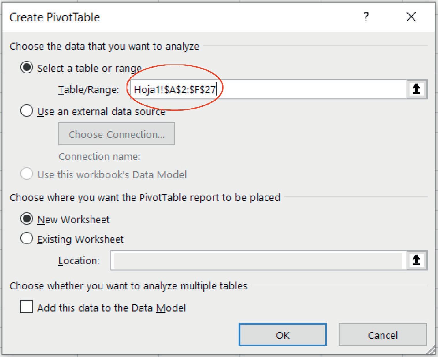
After our table presented in Annex I has been entered in Excel, the Insert tab must be selected from the operations ribbon, and its first option, Pivot Table, as shown in Figure 2.1 below.
Figure 2.1. PivotTable option in the Insert tab
There are two options for entering pivot tables. The first is to perform a prior selection of the data in the original table (see Annex I) to be reported using the pivot table, and then select the Pivot Table option. The second consists of first selecting the Pivot Table option, and in the “Create Dynamic Table” pop-up window that appears, select the range or table of data to report in the analysis, as shown in Figure 2.2 below.
Basic Concepts in Pivot Tables
ISBN: 978-84-18432-98-9
DOI: http://dx.doi.org/10.6035/Sapientia179
13
Beatriz Forés Julián, Alba Puig Denia, Rafael Lapiedra Alcamí, Francisco Fermín Mallén Broch, José Mª Fernández Yáñez
Figure 2.2. Selecting data in the Create PivotTable option

There is another option for selecting data from external sources such as other Excel files, databases and even text files (see Figure 2.3).
Basic Concepts in Pivot Tables
ISBN: 978-84-18432-98-9
Figure 2.3. Use of an external data source
DOI: http://dx.doi.org/10.6035/Sapientia179
14
Beatriz Forés Julián, Alba Puig Denia, Rafael Lapiedra Alcamí, Francisco Fermín Mallén Broch, José Mª Fernández Yáñez
For an existing spreadsheet, the Location must be specified exactly, as shown in Figure 2.4 below. Of the two options available, it is advisable to create a new spreadsheet for the final location of the table in order to avoid possible confusion in the data analyzed. Once the data set has been selected in the previous table, select the location where you want to place the pivot table - in either a New spreadsheet or in the Existing spreadsheet (see Figure 2.4).
Figure 2.4. Choosing where to place the PivotTable

As explained later, more than one pivot table can be used as a data source, which presumes that there are previous relationships between them.
Figure 2.5. Adding more than one PivotTable as a data source

After selecting the option, click on the OK button. Depending on the location of the dynamic table, some pop-up windows will be displayed like those shown in Figure 2.6 below.
15
Basic Concepts in Pivot Tables
ISBN: 978-84-18432-98-9
DOI: http://dx.doi.org/10.6035/Sapientia179
Beatriz Forés Julián, Alba Puig Denia, Rafael Lapiedra Alcamí, Francisco Fermín Mallén Broch, José Mª Fernández YáñezFigure 2.6. PivotTable fields
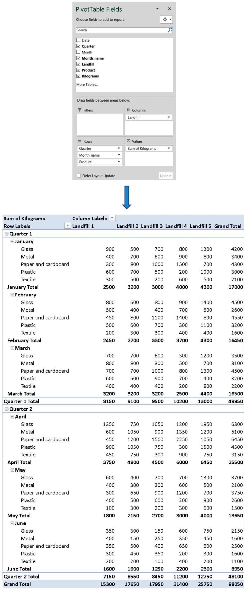
At this point, the pivot table is created with the data selected from the original table (see annex 1). With this pivot table activated, the pop-up window can be accessed (it appears on the right side of the spreadsheet), from where each of the fields for building the dynamic table can be selected, and its distribution chosen from between Columns and Rows (see Figure 2.7). Report Filters can also be applied, and various options selected for calculating the Values, which permit options to be reported including the sum (which will be used in the following examples), the average and the variance. These options will be described in greater detail in section 2.2.
Figure 2.7. Options in the PivotTable Fields


Basic Concepts in Pivot Tables
ISBN: 978-84-18432-98-9
DOI: http://dx.doi.org/10.6035/Sapientia179
16
Beatriz Forés Julián, Alba Puig Denia, Rafael Lapiedra Alcamí, Francisco Fermín Mallén Broch, José Mª Fernández Yáñez
The list of fields in the pivot table includes all the fields that can be used as column labels, row labels, to apply a filter (showing the data based on the selected value), or for a summary function or operation (sum, average, standard deviation, etc.). These fields can be entered in each area by selecting and dragging them.
The order of the existing fields in columns or rows can be changed by moving the previously selected fields with the mouse, or with the options shown in the drop-down in each field, as shown in Figure 2.8. The final Field Configuration option will be explained in greater detail in section 2.2.
Figure 2.8. PivotTable Fields operating options

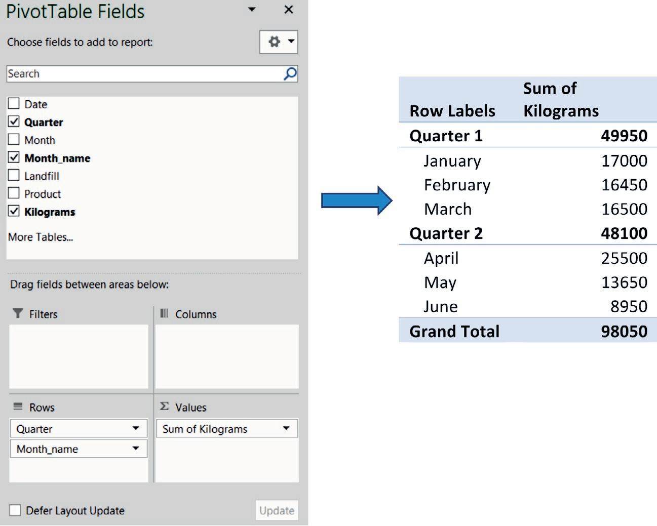
Using the previous options, different tables can be created for the aggregated analysis of the data. Figure 2.9 shows the total kilos recycled per quarter and month, which provides better oversight.
Basic Concepts in Pivot Tables
ISBN: 978-84-18432-98-9
DOI: http://dx.doi.org/10.6035/Sapientia179
17
Beatriz Forés Julián, Alba Puig Denia, Rafael Lapiedra Alcamí, Francisco Fermín Mallén Broch, José Mª Fernández Yáñez
Figure 2.9. Recycling of products in kilos in the first and second quarter
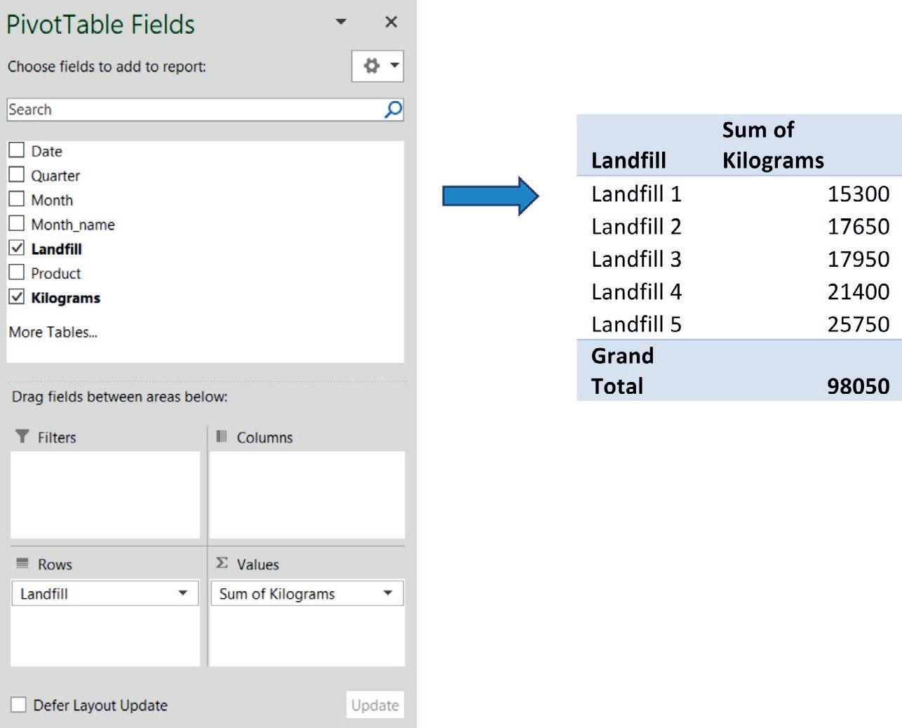
Figure 2.10. Below shows the total kilos added for each landfill.
Figure 2.10. Recycling of products in kilos by landfill
Basic Concepts in Pivot Tables
ISBN: 978-84-18432-98-9
DOI: http://dx.doi.org/10.6035/Sapientia179
18
Beatriz Forés Julián, Alba Puig Denia, Rafael Lapiedra Alcamí, Francisco Fermín Mallén Broch, José Mª Fernández Yáñez
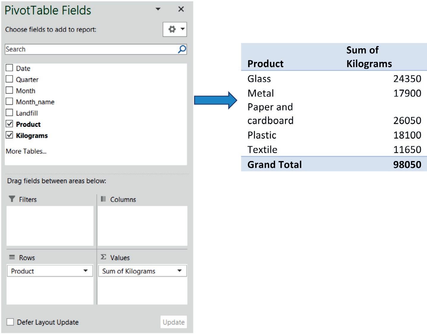
Figure 2.11 shows the kilos recycled by type of product.
Figure 2.11. Recycling of products in kilos by type of product
According to the above data, a little more waste was recycled in the first quarter, the dump with the highest volume of recycling is number 5, and the most recycled product is cardboard.
If we want to do a more detailed analysis, e.g. checking the amount recycled per month of each type of product; the amount recycled per quarter of each product in each landfill, or the type of product that is recycled most each month, a greater level of detail is needed in the data, as shown in Figure 2.12 below.
Basic Concepts in Pivot Tables
ISBN: 978-84-18432-98-9
DOI: http://dx.doi.org/10.6035/Sapientia179
19
Beatriz Forés Julián, Alba Puig Denia, Rafael Lapiedra Alcamí, Francisco Fermín Mallén Broch, José Mª Fernández Yáñez
Figure 2.12.
Basic Concepts in Pivot Tables
ISBN: 978-84-18432-98-9
Recycling
of products in kilos by quarter, month, product, and landfill
DOI: http://dx.doi.org/10.6035/Sapientia179
20
Beatriz Forés Julián, Alba Puig Denia, Rafael Lapiedra Alcamí, Francisco Fermín Mallén Broch, José Mª Fernández Yáñez
The way the data is presented in the following dynamic table is due to the product field being adopted as the main axis of analysis, and it is subsequently completed by the other fields mentioned above (see Figure 2.13).
Figure 2.13. Recycling of products in kilos by quarter, month, product, and landfill
21
Basic Concepts in Pivot Tables

ISBN: 978-84-18432-98-9
DOI: http://dx.doi.org/10.6035/Sapientia179
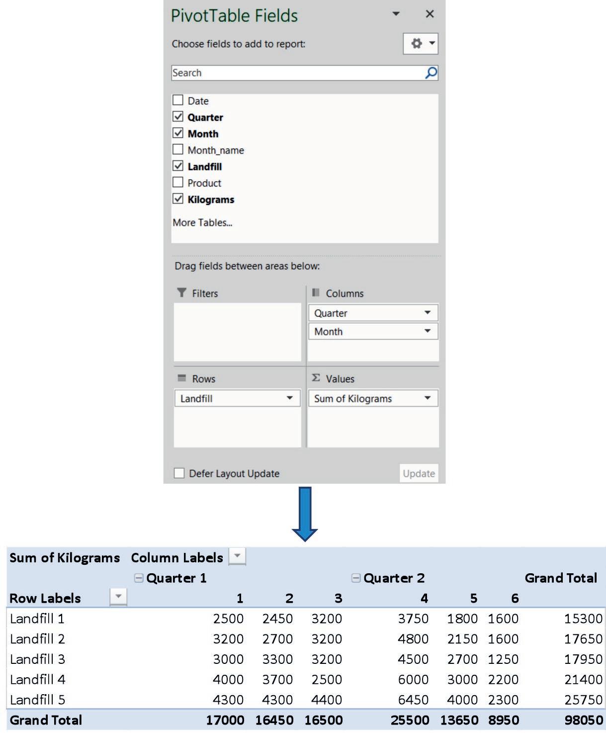
Beatriz Forés Julián, Alba Puig Denia, Rafael Lapiedra Alcamí, Francisco Fermín Mallén Broch, José Mª Fernández YáñezFinally, the following Pivot Table uses the type of landfill as the main criterion for listing the information (see Figure 2.14).
Figure 2.14. Information on recycled kilos, using the landfill of origin as the main criterion
2.2 VALUE FIELD SETTINGS (Σ)
In the Values area in the Pivot Table Fields box, you can select the type of operation to be carried out with the field values, left clicking on the area itself; a new window with all these possibilities will open up (see Figure 2.15).
Basic Concepts in Pivot Tables
ISBN: 978-84-18432-98-9
DOI: http://dx.doi.org/10.6035/Sapientia179
22
Beatriz Forés Julián, Alba Puig Denia, Rafael Lapiedra Alcamí, Francisco Fermín Mallén Broch, José Mª Fernández Yáñez
Figure 2.15. Value Field Settings

The summary of options that appear for the value field includes:
• Sum: calculates the sum of the values, which is the default function to use for numeric values.
• Count : counts the number of non-numeric repeating values. The Count summary function works in the same way as the Count worksheet function. This is the default for non-numeric values.
• Average : calculates the average of the selected values.
• Maximization : shows the maximum value.
• Minimization : shows the minimum value.
• Product : calculates the product of values.
• Count numbers : Count the number of values that are numbers. The summary function count numbers works in the same way as the worksheet function Count
• Standard deviation : calculates the standard deviation of a population, where the sample is a subset of the entire population.
• Typical deviation : calculates the typical deviation of a population, where the population is all the values to be summarized.
• Variance : calculates the variance of a population, where the sample is a subset of the entire population.
• Variance of a population : calculates the variance of a population, where the population is all the values to be summarized.
Basic Concepts in Pivot Tables
ISBN: 978-84-18432-98-9
DOI: http://dx.doi.org/10.6035/Sapientia179
23
Beatriz Forés Julián, Alba Puig Denia, Rafael Lapiedra Alcamí, Francisco Fermín Mallén Broch, José Mª Fernández Yáñez
Another option that is allowed from this window is the Configuration of the field value ; the name of a field in the pivot table can be changed using the Customized name option, although these cannot be repeated (see Figure 2.16).

The Show values tab indicates how the data can be presented in percentages of the columns or rows, or related to another field (see Figure 2.16).
Figure 2.16. Value Field options to be showed
The options that can be chosen from the Show values drop-down menu are shown in Tables 2.1-2.9 below.
Table 2.1. % of the general total
Sum of Kilograms Month
Landfill 1 2 3 4 5 6 Grand Total
Landfill 1 2.55% 2.50% 3.26% 3.82% 1.84% 1.63% 15.60%
Landfill 2 3.26% 2.75% 3.26% 4.90% 2.19% 1.63% 18.00%
Landfill 3 3.06% 3.37% 3.26% 4.59% 2.75% 1.27% 18.31%
Landfill 4 4.08% 3.77% 2.55% 6.12% 3.06% 2.24% 21.83%
Landfill 5 4.39% 4.39% 4.49% 6.58% 4.08% 2.35% 26.26%
Grand Total 17.34% 16.78% 16.83% 26.01% 13.92% 9.13% 100.00%
24
Basic Concepts in Pivot Tables
ISBN: 978-84-18432-98-9
DOI: http://dx.doi.org/10.6035/Sapientia179
Beatriz Forés Julián, Alba Puig Denia, Rafael Lapiedra Alcamí, Francisco Fermín Mallén Broch, José Mª Fernández YáñezTable 2.2. % of the total number of columns
Sum of Kilograms Month
Landfill
1 2 3 4 5 6 Grand Total
Landfill 1 14.71% 14.89% 19.39% 14.71% 13.19% 17.88% 15.60%
Landfill 2 18.82% 16.41% 19.39% 18.82% 15.75% 17.88% 18.00%
Landfill 3 17.65% 20.06% 19.39% 17.65% 19.78% 13.97% 18.31%
Landfill 4 23.53% 22.49% 15.15% 23.53% 21.98% 24.58% 21.83%
Landfill 5 25.29% 26.14% 26.67% 25.29% 29.30% 25.70% 26.26%
Grand Total 100.00% 100.00% 100.00% 100.00% 100.00% 100.00% 100.00%
Table 2.3. % of the total number of rows
Sum of Kilograms Month
Landfill
1 2 3 4 5 6 Grand Total
Landfill 1 16.34% 16.01% 20.92% 24.51% 11.76% 10.46% 100.00%
Landfill 2 18.13% 15.30% 18.13% 27.20% 12.18% 9.07% 100.00%
Landfill 3 16.71% 18.38% 17.83% 25.07% 15.04% 6.96% 100.00%
Landfill 4 18.69% 17.29% 11.68% 28.04% 14.02% 10.28% 100.00%
Landfill 5 16.70% 16.70% 17.09% 25.05% 15.53% 8.93% 100.00%
Grand Total 17.34% 16.78% 16.83% 26.01% 13.92% 9.13% 100.00%
Table 2.4. % of previous month value
Sum of Kilograms Month
Landfill
1 2 3 4 5 6 Grand Total
Landfill 1 100.00% 98.00% 130.61% 117.19% 48.00% 88.89% Landfill 2 100.00% 84.38% 118.52% 150.00% 44.79% 74.42% Landfill 3 100.00% 110.00% 96.97% 140.63% 60.00% 46.30%
Landfill 4 100.00% 92.50% 67.57% 240.00% 50.00% 73.33% Landfill 5 100.00% 100.00% 102.33% 146.59% 62.02% 57.50%
Grand Total 100.00% 96.76% 100.30% 154.55% 53.53% 65.57%
25
Basic Concepts in Pivot Tables
ISBN: 978-84-18432-98-9
DOI: http://dx.doi.org/10.6035/Sapientia179
Table 2.5. Total in landfill
Sum of Kilograms Month
Landfill
Table 2.6. % of total main rows
1 2 3 4 5 6 Grand Total
Landfill 1 14.71% 14.89% 19.39% 14.71% 13.19% 17.88% 15.60% Landfill 2 18.82% 16.41% 19.39% 18.82% 15.75% 17.88% 18.00% Landfill 3 17.65% 20.06% 19.39% 17.65% 19.78% 13.97% 18.31%
Landfill 4 23.53% 22.49% 15.15% 23.53% 21.98% 24.58% 21.83% Landfill 5 25.29% 26.14% 26.67% 25.29% 29.30% 25.70% 26.26%
Grand Total 100.00% 100.00% 100.00% 100.00% 100.00% 100.00% 100.00%
Table 2.7. % of total main columns
Sum of Kilograms Month
Landfill
1 2 3 4 5 6 Grand Total
Landfill 1 16.34% 16.01% 20.92% 24.51% 11.76% 10.46% 100.00%
Landfill 2 18.13% 15.30% 18.13% 27.20% 12.18% 9.07% 100.00%
Landfill 3 16.71% 18.38% 17.83% 25.07% 15.04% 6.96% 100.00%
Landfill 4 18.69% 17.29% 11.68% 28.04% 14.02% 10.28% 100.00%
Landfill 5 16.70% 16.70% 17.09% 25.05% 15.53% 8.93% 100.00%
Grand Total 17.34% 16.78% 16.83% 26.01% 13.92% 9.13% 100.00%
26
Basic Concepts in Pivot Tables

ISBN: 978-84-18432-98-9
DOI: http://dx.doi.org/10.6035/Sapientia179
Beatriz Forés Julián, Alba Puig Denia, Rafael Lapiedra Alcamí, Francisco Fermín Mallén Broch, José Mª Fernández YáñezTable 2.8. % of total in landfill
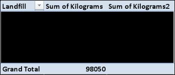
Table 2.9. Sort from highest to lowest
Landfill Sum of Kilograms Sum of Kilograms2
Landfill 1 15300 5 Landfill 2 17650 4 Landfill 3 17950 3 Landfill 4 21400 2 Landfill 5 25750 1 Grand Total 98050
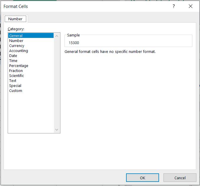
In the Value field window, it is also possible to modify the way in which the numbers are formatted, such as the number of decimal places, the use of the thousand’s separator, the format of negative numbers, etc. using the Number Format option (see Figure 2.17).
Basic Concepts in Pivot Tables
ISBN: 978-84-18432-98-9
DOI: http://dx.doi.org/10.6035/Sapientia179
27
Beatriz Forés Julián, Alba Puig Denia, Rafael Lapiedra Alcamí, Francisco Fermín Mallén Broch, José Mª Fernández Yáñez
Figure 2.17. Format Cells
Finally, the configuration of a value field can also be changed; to do this, go to the field itself in the pivot table and select the Configuration of the value field option on the operations ribbon in the Analyze tab (see Figure 2.18).
Basic Concepts in Pivot Tables

ISBN: 978-84-18432-98-9
Figure 2.18. Value Field Settings in the Analyze tab
DOI: http://dx.doi.org/10.6035/Sapientia179
28
Beatriz Forés Julián, Alba Puig Denia, Rafael Lapiedra Alcamí, Francisco Fermín Mallén Broch, José Mª Fernández Yáñez
2 .3 . FIELD OPTIONS: ROWS, COLUMNS AND FILTERS
2.3.1. Configuration of a non-value field from an active field
The Field Configuration option can be accessed from the pivot table itself, by clicking the right mouse button on a data field (normally entered as row or column labels).
The options that appear under Field Configuration , which in this case are a non-value type, are shown in Figure 2.19 below.
Note:
The Custom Name can rename one field for another (as long as it is not repeated).
Figure 2.19. Non-value field setting
29
Basic Concepts in Pivot Tables
ISBN: 978-84-18432-98-9
DOI: http://dx.doi.org/10.6035/Sapientia179
Beatriz Forés Julián, Alba Puig Denia, Rafael Lapiedra Alcamí, Francisco Fermín Mallén Broch, José Mª Fernández YáñezFrom the Subtotals tab, the Subtotals option can be selected, with three possibilities:
• Automatic, showing the subtotal.
• None, showing the field without any subtotal.
• Customized, allowing a choice between different functions (see Figure 2.20).
Another option that appears on the Subtotals and Filters tab is Filter , which allows users to include new items in a Pivot Table report with a filter already applied. This option must be enabled if filters are used in this field.

This option must be checked so that the new fields that are added to any pivot table (previously updated from the Analyze tab) can be used as filters.
Figure 2.20. Field Settings, Subtotals and Filters tab
The following functions can be accessed by selecting the Design and Printing tab:
Basic Concepts in Pivot Tables
ISBN: 978-84-18432-98-9
DOI: http://dx.doi.org/10.6035/Sapientia179
30
Beatriz Forés Julián, Alba Puig Denia, Rafael Lapiedra Alcamí, Francisco Fermín Mallén Broch, José Mª Fernández Yáñez
Show item labels in schematic format
This option enables or disables the generic field label to be changed in the next field label in the same column (compact form) (see Figure 2.21).

Figure 2.21. Display labels from the next field in the same column and results from the selection
31

Basic Concepts in Pivot Tables
ISBN: 978-84-18432-98-9
DOI: http://dx.doi.org/10.6035/Sapientia179
Beatriz Forés Julián, Alba Puig Denia, Rafael Lapiedra Alcamí, Francisco Fermín Mallén Broch, José Mª Fernández YáñezThis option also includes the possibility of showing subtotals at the top of each group, by adding a new row.
Sum of Kilograms
Landfill Product
Month
1 2 3 4 5 6 Grand Total
Landfill 1 2500 2450 3200 3750 1800 1600 15300 Glass 900 800 700 1350 600 350 4700 Metal 400 500 800 600 400 400 3100 Paper and cardboard 300 450 700 450 300 350 2550 Plastic 600 500 600 900 400 300 3300 Textile 300 200 400 450 100 200 1650 Landfill 2 3200 2700 3200 4800 2150 1600 17650 Glass 500 600 700 750 400 300 3250 Metal 700 400 800 1050 300 150 3400 Paper and cardboard 800 800 700 1200 650 500 4650 Plastic 700 600 600 1050 500 450 3900 Textile 500 300 400 750 300 200 2450 Landfill 3 3000 3300 3200 4500 2700 1250 17950 Glass 700 800 600 1050 700 150 4000 Metal 600 400 300 900 300 250 2750 Paper and cardboard 1000 1100 1000 1500 900 400 5900 Plastic 500 700 900 750 600 350 3800 Textile 200 300 400 300 200 100 1500 Landfill 4 4000 3700 2500 6000 3000 2200 21400 Glass 800 900 300 1200 700 600 4500 Metal 900 700 500 1350 600 350 4400
Paper and cardboard 1500 1400 800 2250 1200 650 7800 Plastic 200 300 700 300 200 200 1900 Textile 600 400 200 900 300 400 2800 Landfill 5 4300 4300 4400 6450 4000 2300 25750 Glass 1300 1400 1200 1950 1300 750 7900 Metal 800 600 700 1200 500 450 4250 Paper and cardboard 700 800 1300 1050 700 600 5150 Plastic 1000 1100 400 1500 900 300 5200 Textile 500 400 800 750 600 200 3250
Grand Total 17000 16450 16500 25500 13650 8950 98050
Figure 2.22. Display subtotals at the top of each group and results from its selection
Basic Concepts in Pivot Tables

ISBN: 978-84-18432-98-9
DOI: http://dx.doi.org/10.6035/Sapientia179
32
Beatriz Forés Julián, Alba Puig Denia, Rafael Lapiedra Alcamí, Francisco Fermín Mallén Broch, José Mª Fernández Yáñez
Show item labels in tabular format
When this box is enabled, the elements of the fields are arranged in tabular form. This setting only applies to the fields located within the row labels area (see Figure 2.23).
Figure 2.23. Show item labels in tabular forms
Other design and printing options:
Other actions in this tab are:
1. Repeat item labels.
2. Insert blank line after each item and increase the space, e.g. before the presentation of subtotals.
3. Show pivot table elements that do not contain data.
4. Insert a page break after each item when printing the pivot table.

Basic Concepts in Pivot Tables
ISBN: 978-84-18432-98-9
DOI: http://dx.doi.org/10.6035/Sapientia179
33
Beatriz Forés Julián, Alba Puig Denia, Rafael Lapiedra Alcamí, Francisco Fermín Mallén Broch, José Mª Fernández Yáñez
2 .4 . AGGREGATE OPTION
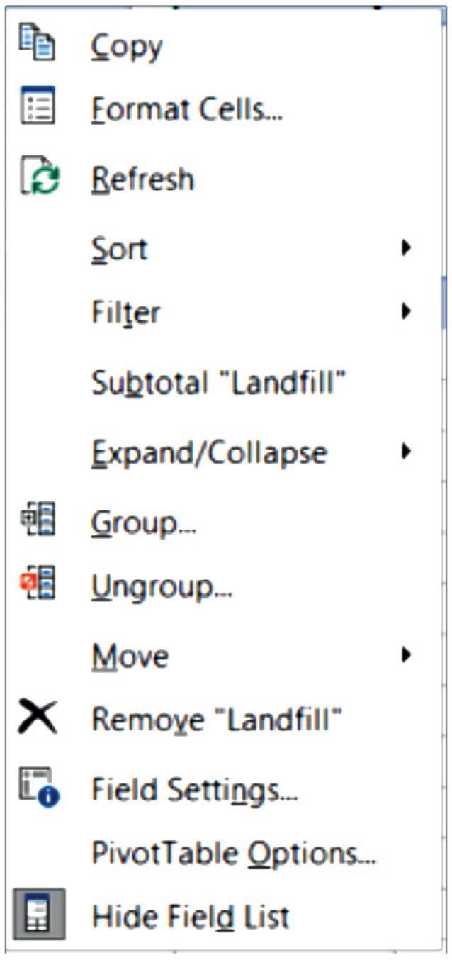
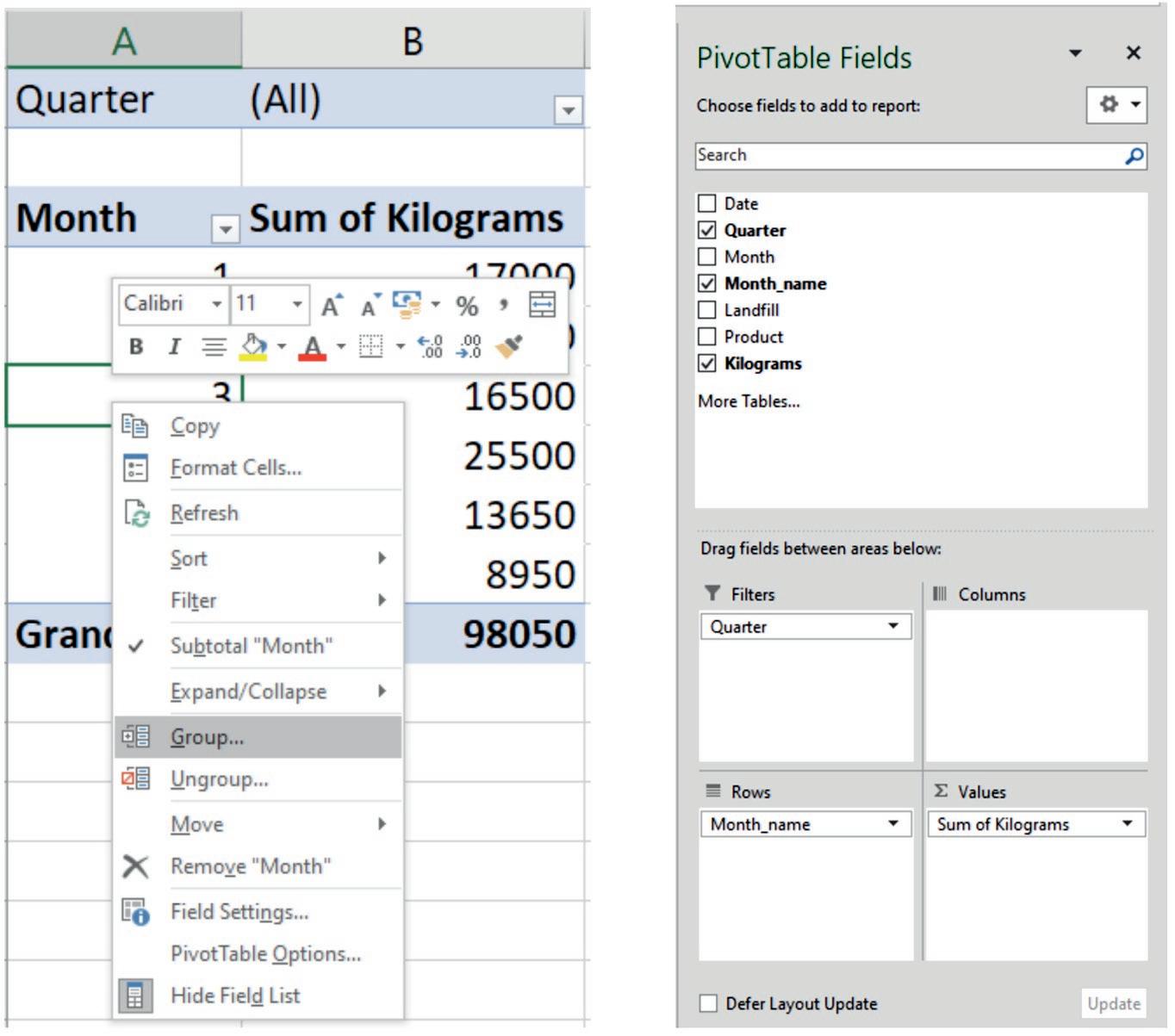
By selecting on the pivot table itself and clicking the right button of the mouse, the Group option appears (see Figure 2.24). In this case, we will work with the example of the pivot table that accompanies the Figure below.
Figure 2.24. Group Option
There is the option to group or ungroup data using the Group selection option when they meet the condition to be grouped, e.g. when they belong to the same detailed category. In this case, the months can be presented by quarter.
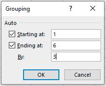
The months can be grouped into two quarters by selecting the option to aggregate months in groups of three, as shown in Figure 2.25 below.
Basic Concepts in Pivot Tables
ISBN: 978-84-18432-98-9
DOI: http://dx.doi.org/10.6035/Sapientia179
34
Beatriz Forés Julián, Alba Puig Denia, Rafael Lapiedra Alcamí, Francisco Fermín Mallén Broch, José Mª Fernández Yáñez
Figure 2.25. Grouping
Table 2.10 is presented with the arrangement shown in Figure 2.25.
2.10. Grouping of kilos by quarters
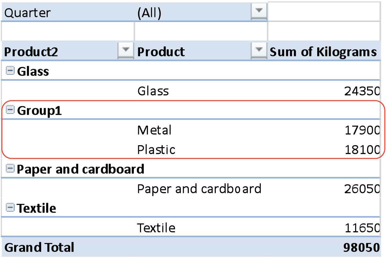
The Ungroup option is used to break up a group. Another example of fields grouping would be the one shown in Table 2.11, which presents the grouping of two products, Metal and Plastic, in the same group.
Basic Concepts in Pivot Tables
ISBN: 978-84-18432-98-9
DOI: http://dx.doi.org/10.6035/Sapientia179
35
Beatriz Forés Julián, Alba Puig Denia, Rafael Lapiedra Alcamí, Francisco Fermín Mallén Broch, José Mª Fernández Yáñez
Table
Quarter (All) Month Sum of Kilograms 1-3 49950 4-6 48100 Grand Total 98050
Table 2.11. Grouping two types of waste in the same group
2 .5 . INSERTING A TIMESCALE
This option allows a timescale to be used to display data from different time periods, making it comparison easy. In order to use this option, a new column is introduced in the main table (see Annex I) with the accurate dates for each entry.
This requires changes to the data in the pivot table itself so that this new Date field is added. The data is not updated, because we are not adding new records (rows) - we are instead adding new fields (columns). To change the source of the table, select the option Change data source that appears in the Analyze tab, and then select all the desired information (see Figure 2.26).
Basic Concepts in Pivot Tables
ISBN: 978-84-18432-98-9
Figure 2.26. Change PivotTable Data Source
DOI: http://dx.doi.org/10.6035/Sapientia179

36
Beatriz Forés Julián, Alba Puig Denia, Rafael Lapiedra Alcamí, Francisco Fermín Mallén Broch, José Mª Fernández Yáñez
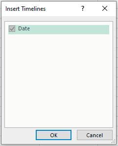
After this new field has been added to the table, click on the Insert timeline option that appears on the Insert tab, in the Filters section.

Figure 2.27. Timeline
The following window for inserting a timeline will appear (see Figure 2.28).
Figure 2.28. Insert Timelines
The Date option must be selected and this window will appear. The data can be filtered by the period of time selected (see Figure 2.29).
37
Basic Concepts in Pivot Tables
ISBN: 978-84-18432-98-9
DOI: http://dx.doi.org/10.6035/Sapientia179
Beatriz Forés Julián, Alba Puig Denia, Rafael Lapiedra Alcamí, Francisco Fermín Mallén Broch, José Mª Fernández YáñezFigure 2.29. Selecting the date to filter the data


For example, using the selection shown in Figure 2.30 below, we can filter the data to obtain only those for the second quarter.
Basic Concepts in Pivot Tables
ISBN: 978-84-18432-98-9
Figure 2.30. Second quarter data selection example
DOI: http://dx.doi.org/10.6035/Sapientia179
38
Beatriz Forés Julián, Alba Puig Denia, Rafael Lapiedra Alcamí, Francisco Fermín Mallén Broch, José Mª Fernández Yáñez
Chapter 3: Direct menu options in a pivot table
3 .1 . SORT
The Sort option allows users to insert an order in the data. An example pivot table must first be created in order to work with this option (see Table 3.1).
Table 3.1. Starting pivot table example
Product Sum of Kilograms
Glass 24350 Metal 17900 Paper and cardboard 26050 Plastic 18100 Textile 11650 Grand Total 98050
By selecting the pivot table and the field to be ordered (in this case the sum of kilograms), and clicking on the right button, Excel displays the Sort options shown in Figure 3.1 below.
Basic Concepts in Pivot Tables
ISBN: 978-84-18432-98-9
DOI: http://dx.doi.org/10.6035/Sapientia179
39
Beatriz Forés Julián, Alba Puig Denia, Rafael Lapiedra Alcamí, Francisco Fermín Mallén Broch, José Mª Fernández Yáñez
Figure 3.1. Sorting options
Basic Concepts in Pivot Tables
ISBN:

40
978-84-18432-98-9 Beatriz Forés Julián, Alba Puig Denia, Rafael Lapiedra Alcamí, Francisco Fermín Mallén Broch, José Mª Fernández Yáñez DOI: http://dx.doi.org/10.6035/Sapientia179
text type fields are
product
Table 3.2. Sorting the text field in alphabetically descending order Product Sum of Kilograms Glass 24350 Metal 17900 Paper and cardboard 26050 Plastic 18100 Textile 11650 Grand Total 98050
access More Sort Options , the dialog box allows users to select between the options shown
below. In this dialog you can access More Options, when the
data
a value field (e.g. kilos).
If
selected (the
type field in our example), the sort from lowest to highest becomes descending or ascending (see Table 3.2).
To
in Figure 3.2
selected previous
is
Figure 3.2. More Sort Options dialog box

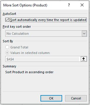
The More Sort Options (see Figure 3.3) allows the user to enter automatic sorting options every time the report is updated.
Figure 3.3. More Sort Options
41
Basic Concepts in Pivot Tables
ISBN: 978-84-18432-98-9
DOI: http://dx.doi.org/10.6035/Sapientia179
Beatriz Forés Julián, Alba Puig Denia, Rafael Lapiedra Alcamí, Francisco Fermín Mallén Broch, José Mª Fernández Yáñez3.2. OTHER OPTIONS IN THE DROP-DOWN MENU
By clicking on the data in any of the pivot tables created with the right button of the mouse, Excel shows a submenu that contains various options, including those for basic formatting. Most of these options have been discussed previously, so they will not be explained again.
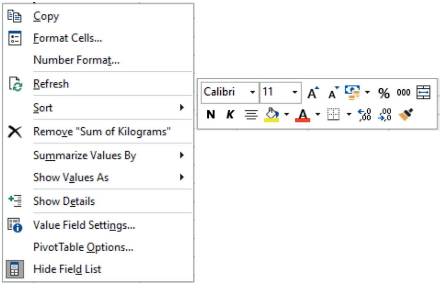
When a value field is selected, the options that appear are those shown in Figure 3.4 below, while other options are added for non-value fields (e.g. landfill), as shown in Figure 3.5.
Basic Concepts in Pivot Tables
ISBN: 978-84-18432-98-9
Figure 3.4. Options for non-value fields
42
DOI: http://dx.doi.org/10.6035/Sapientia179
Beatriz Forés Julián, Alba Puig Denia, Rafael Lapiedra Alcamí, Francisco Fermín Mallén Broch, José Mª Fernández YáñezFigure 3.5. Options for non-value fields
3 .3 . DATA FILTER OPTIONS WITHIN FIELDS
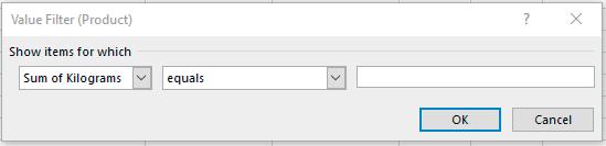
The Filter option is shown for this type of non-value field. This filter option is not related to the option shown in the Subtotals and Filters tab to show the fields, and nor is it related to the Filter area in the pivot table related to entering a grouping level in the table, as it shows the data in the fields that meet a condition: being in the top 10 (see Figure 3.6), according to the label’s values (see Figure 3.7) and by the value of a field (see Figure 3.8).

Figure 3.6. Top 10 Filter

Basic Concepts in Pivot Tables
ISBN: 978-84-18432-98-9
DOI: http://dx.doi.org/10.6035/Sapientia179
43
Beatriz Forés Julián, Alba Puig Denia, Rafael Lapiedra Alcamí, Francisco Fermín Mallén Broch, José Mª Fernández Yáñez
Figure 3.7. Label Filter
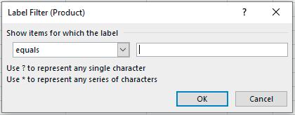
Figure 3.8. Value Filter
Finally, we will introduce a new Search Filter to quickly and efficiently access specific product data in large spreadsheets. This type of filter is interactive, as it allows the user to search for the data and make selections according to the element searched. Wildcards can be used, such as an asterisk to search for related names, for example, Castell *; in this case the search would return names such as Castellón, Castellfort and Castellnovo. This filter is applied using the dropdown, in the field shown in Figure 3.9.
Basic Concepts in Pivot Tables
ISBN: 978-84-18432-98-9
DOI: http://dx.doi.org/10.6035/Sapientia179
44
Beatriz Forés Julián, Alba Puig Denia, Rafael Lapiedra Alcamí, Francisco Fermín Mallén Broch, José Mª Fernández Yáñez
Basic Concepts in Pivot Tables

ISBN: 978-84-18432-98-9
Figure 3.9. Search filter for a field
DOI: http://dx.doi.org/10.6035/Sapientia179
45
Beatriz Forés Julián, Alba Puig Denia, Rafael Lapiedra Alcamí, Francisco Fermín Mallén Broch, José Mª Fernández Yáñez
Chapter 4: Analyze menu options
4 .1 . ACTIONS IN THE PIVOT TABLE
Finally, as with any Excel component, you can perform various actions such as Clear, Select and Move Pivot Table (see Figure 4.1).


Figure 4.1. Pivot table Actions
4 .1 .1 . Delete actions
Figure 4.2. displays the Clear options table.
Basic Concepts in Pivot Tables
ISBN: 978-84-18432-98-9
Figure 4.2. Clear options
47
DOI: http://dx.doi.org/10.6035/Sapientia179
Beatriz Forés Julián, Alba Puig Denia, Rafael Lapiedra Alcamí, Francisco Fermín Mallén Broch, José Mª Fernández YáñezClear All : removes all data from the pivot table, including fields, formatting, and filters.
Clear filters : removes the filters entered.
4 .1 .2 . The Select action
The Select action is used to select an item from the pivot table. It is important that the pivot table is selected so that all selection options are displayed. Labels and Values, Values and Labels are the options that can be selected (see Figure 4.3).
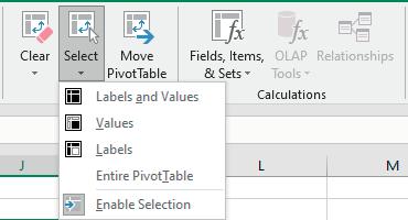
Figure 4.3. Selection options
4 .1 .3 The Move table action
Move Pivot Table moves the pivot table to a location in the workbook that is being used, as shown in Figure 4.4.
Figure 4.4. Move Pivot Table

Basic Concepts in Pivot Tables
ISBN: 978-84-18432-98-9
DOI: http://dx.doi.org/10.6035/Sapientia179
48
Beatriz Forés Julián, Alba Puig Denia, Rafael Lapiedra Alcamí, Francisco Fermín Mallén Broch, José Mª Fernández Yáñez
4 .2 . CALCULATIONS
The Analyze tab also includes the Calculations section, which has actions which will be described below (see Figure 4.5).
Figure 4.5. Calculations
4 .2 .1 . Fields, Items and Sets
The Fields, Items & Sets option allows the calculated fields and elements in a pivot table to be created and modified (see Figure 4.6).

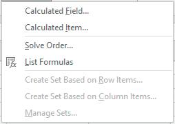
Figure 4.6. Fields, Items & Sets
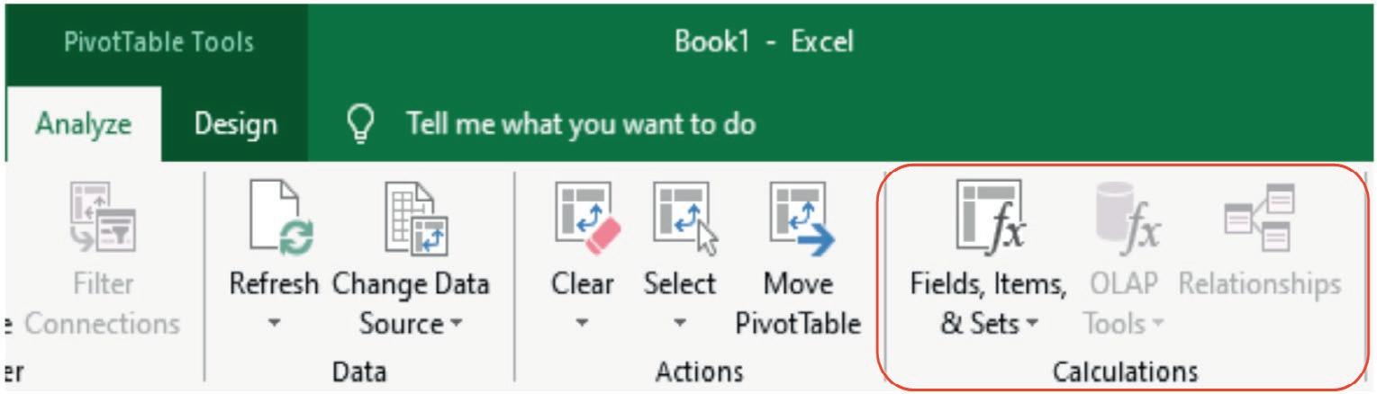
Figure 4.7. Calculated Field
Basic Concepts in Pivot Tables
ISBN: 978-84-18432-98-9
DOI: http://dx.doi.org/10.6035/Sapientia179
49
Beatriz Forés Julián, Alba Puig Denia, Rafael Lapiedra Alcamí, Francisco Fermín Mallén Broch, José Mª Fernández Yáñez
For example, to make a forecast for the kilos recycled in the third semester (now the data only report information for two semesters), we could estimate that in the second quarter sales will increase by 5%. In order to apply this calculated field option, the following pivot table should first be entered (see Table 4.1).
Table 4.1. Pivot table with data for kilos recycled in the second quarter and product type
Sum of Kilograms Quarter
Product Quarter 2
Glass 12150 Metal 8800 Paper and cardboard 12700 Plastic 8700 Textile 5750 Grand Total 48100
If the pivot table and the Calculated Field option in Fields, Items & sets are selected, the dialog box below will appear (see Figure 4.8).
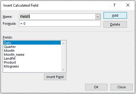
Figure 4.8. Insert Calculated Field
50
Basic Concepts in Pivot Tables
ISBN: 978-84-18432-98-9
DOI: http://dx.doi.org/10.6035/Sapientia179
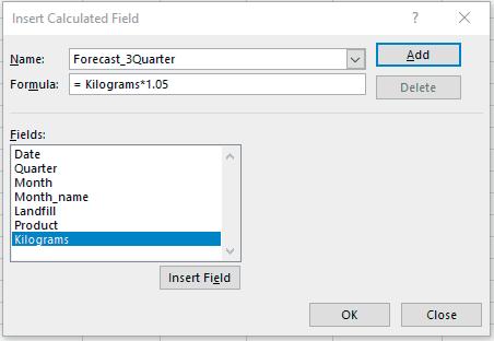
Beatriz Forés Julián, Alba Puig Denia, Rafael Lapiedra Alcamí, Francisco Fermín Mallén Broch, José Mª Fernández YáñezYou should enter a name for this Field1 . In this case, it identifies the sales forecast for the third quarter. Insert the kilos field in the formula, and multiply them by 1.05 to increase them by 5%, and then Accept (see Figure 4.9).
Figure 4.9. Calculated field customization
The result of creating this calculated field is shown in Table 4.2 below.
Table 4.2. Sales forecast in the third quarter
51
Basic Concepts in Pivot Tables
ISBN: 978-84-18432-98-9
DOI: http://dx.doi.org/10.6035/Sapientia179
Beatriz Forés Julián, Alba Puig Denia, Rafael Lapiedra Alcamí, Francisco Fermín Mallén Broch, José Mª Fernández YáñezQuarter Values Quarter 2 Product Sum of Kilograms Sum of Forecast_3Quarter Glass 12150 12757.5 Metal 8800 9240 Paper and cardboard 12700 13335 Plastic 8700 9135 Textile 5750 6037.5 Grand Total 48100 50505
If you want to delete a calculated field, you should select the field that contains the element to be deleted. On the Options tab, in the Tools group, click on Formulas , and then click on Calculated Field . In the Name field, select the element to delete, and click on Delete (see Figure 4.10).
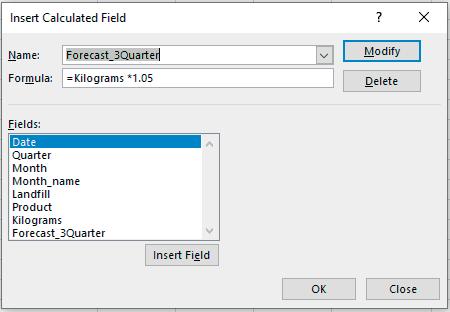

Figure 4.10. Delete calculated field
4 .2 .2 . Calculated Item option
A Calculated Item allows you to add a new record or row to the source of the data, by entering a formula that takes the data from other rows (see Figure 4.11).
Figure 4.11. Calculated Item option
Basic Concepts in Pivot Tables
ISBN: 978-84-18432-98-9
DOI: http://dx.doi.org/10.6035/Sapientia179
52
Beatriz Forés Julián, Alba Puig Denia, Rafael Lapiedra Alcamí, Francisco Fermín Mallén Broch, José Mª Fernández Yáñez
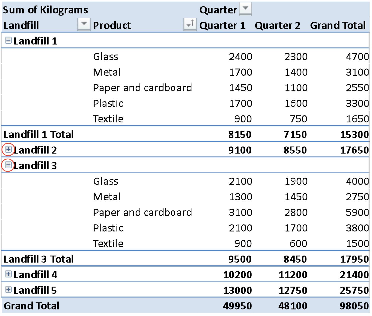
To do this, the pivot table below should be entered, which will provide the basis for the rest of the calculations (see Table 4.3).
Table 4.3. Initial pivot table with the sum of kilos for each zone and quarter
Sum of Kilograms Quarter
Landfill Quarter 1 Quarter 2 Grand Total
Landfill 1 8150 7150 15300 Landfill 2 9100 8550 17650 Landfill 3 9500 8450 17950
Landfill 4 10200 11200 21400 Landfill 5 13000 12750 25750
Grand Total 49950 48100 98050
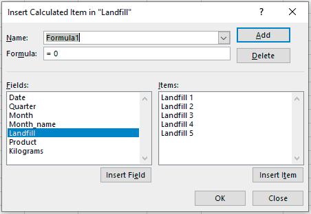
First, place the cursor in a field that can be used as a calculated field (the landfill field in this case). After selecting the pivot table, click on the option Calculated Item entered previously (Figure 4.11). The box dialog below will then appear (see Figure 4.12).
Basic Concepts in Pivot Tables
ISBN: 978-84-18432-98-9
Figure 4.12. Insert Calculated Item in ‘Landfill’
DOI: http://dx.doi.org/10.6035/Sapientia179
53
Beatriz Forés Julián, Alba Puig Denia, Rafael Lapiedra Alcamí, Francisco Fermín Mallén Broch, José Mª Fernández Yáñez
In this case, a new formula will be created to obtain 15% of the kilos of recycled product each quarter; the name of the field will be “Increase over the quarter” (see Figure 4.13).
Figure 4.13. Calculated item customization
As a result, a new row of data will be obtained with 15% of the kilos of each quarter from all the landfills (see Table 4.4). Table 4.4. Row with the assigned

Basic Concepts in Pivot Tables
ISBN: 978-84-18432-98-9
DOI: http://dx.doi.org/10.6035/Sapientia179
54
Beatriz Forés Julián, Alba Puig Denia, Rafael Lapiedra Alcamí, Francisco Fermín Mallén Broch, José Mª Fernández Yáñez
Sum of Kilograms Quarter Landfill Quarter 1 Quarter 2 Grand Total Landfill 1 8150 7150 15300 Landfill 2 9100 8550 17650 Landfill 3 9500 8450 17950 Landfill 4 10200 11200 21400 Landfill 5 13000 12750 25750 Increase over the quarter 7492.5 7215 14707.5 Grand Total 57442.5 55315 112757.5
quarterly increase
To delete a calculated element, click on the field that contains the element to be deleted, and on the Options tab, in the Tools group, select Formulas , Calculated Item , in the same way as previously when deleting a calculated field (see Figure 4.10). In the Name option, select the element to delete, and press the Delete button.
4 .3 . ANALYZE MENU TOOLS
This tab contains two main sections - Pivot Chart and Recommended Pivot Tables , as shown in Figure 4.14 below.
Figure 4.14. Tools
The Pivot Chart option creates charts based on the data in the pivot table the user is working with.
The Recommended Pivot Tables option provides a series of recommended pivot tables that can be created from the source data (see Figure 4.15).

55
Basic Concepts in Pivot Tables
ISBN: 978-84-18432-98-9
DOI: http://dx.doi.org/10.6035/Sapientia179
Beatriz Forés Julián, Alba Puig Denia, Rafael Lapiedra Alcamí, Francisco Fermín Mallén Broch, José Mª Fernández YáñezISBN: 978-84-18432-98-9

56
Basic Concepts in Pivot Tables
Beatriz Forés Julián, Alba Puig Denia, Rafael Lapiedra Alcamí, Francisco Fermín Mallén Broch, José Mª Fernández Yáñez DOI:
Sum of Kilograms Quarter Landfill Product Quarter 1 Quarter 2 Grand Total Landfill 1 Glass 2400 2300 4700 Metal 1700 1400 3100 Paper and cardboard 1450 1100 2550 Plastic 1700 1600 3300 Textile 900 750 1650 Landfill 1 Total 8150 7150 15300 Landfill 2 9100 8550 17650 Landfill 3 9500 8450 17950 Landfill 4 10200 11200 21400 Landfill 5 13000 12750 25750 Grand Total 49950 48100 98050
Recommended
Tables
http://dx.doi.org/10.6035/Sapientia179
Figure 4.15.
Pivot
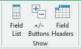
4 .4 . SHOW
In this section, we will discuss the functionalities grouped in the Show tab (see Figure 4.16).
Figure 4.16. Controls on the Show tab
The options appearing in this group of controls are:
1. Field List , which shows or hides the list of fields and allows the user to add and remove fields in the pivot table being worked on (see Figure 4.17).
Figure 4.17. Pivot table controls

57
Basic Concepts in Pivot Tables
ISBN: 978-84-18432-98-9
DOI: http://dx.doi.org/10.6035/Sapientia179
Beatriz Forés Julián, Alba Puig Denia, Rafael Lapiedra Alcamí, Francisco Fermín Mallén Broch, José Mª Fernández Yáñez2. +/- Buttons Shows , which shows or hides the elements in a pivot table (see Table 4.5).
Table 4.5. Show or hide elements
3. Field Headers , which shows or hides the headings in a pivot table by rows and columns.
Tables 4.6 and 4.7 show different types of headings.
Basic Concepts in Pivot Tables
ISBN: 978-84-18432-98-9
DOI: http://dx.doi.org/10.6035/Sapientia179
58
Beatriz Forés Julián, Alba Puig Denia, Rafael Lapiedra Alcamí, Francisco Fermín Mallén Broch, José Mª Fernández Yáñez
Table 4.6. Example of a pivot table with headers
Sum of Kilograms
Quarter
Landfill Product Quarter 1 Quarter 2 Grand Total
Landfill 1
Glass 2400 2300 4700
Metal 1700 1400 3100 Paper and cardboard 1450 1100 2550 Plastic 1700 1600 3300 Textile 900 750 1650
Landfill 1 Total 8150 7150 15300 Landfill 2
Glass 1800 1450 3250 Metal 1900 1500 3400 Paper and cardboard 2300 2350 4650 Plastic 1900 2000 3900 Textile 1200 1250 2450
Landfill 2 Total 9100 8550 17650 Landfill 3 9500 8450 17950 Landfill 4 10200 11200 21400 Landfill 5 13000 12750 25750 Grand Total 49950 48100 98050
Basic Concepts in Pivot Tables
ISBN: 978-84-18432-98-9
DOI: http://dx.doi.org/10.6035/Sapientia179
59
Beatriz Forés Julián, Alba Puig Denia, Rafael Lapiedra Alcamí, Francisco Fermín Mallén Broch, José Mª Fernández Yáñez
Table 4.7. Example of a pivot table without headers
Sum of Kilograms
Landfill 1
Quarter 1 Quarter 2 Grand Total
Glass 2400 2300 4700 Metal 1700 1400 3100 Paper and cardboard 1450 1100 2550 Plastic 1700 1600 3300 Textile 900 750 1650
Landfill 1 Total 8150 7150 15300 Landfill 2
Glass 1800 1450 3250 Metal 1900 1500 3400 Paper and cardboard 2300 2350 4650 Plastic 1900 2000 3900 Textile 1200 1250 2450
Landfill 2 Total 9100 8550 17650 Landfill 3 9500 8450 17950 Landfill 4 10200 11200 21400 Landfill 5 13000 12750 25750
Grand Total 49950 48100 98050
60
Basic Concepts in Pivot Tables
ISBN: 978-84-18432-98-9
DOI: http://dx.doi.org/10.6035/Sapientia179
Beatriz Forés Julián, Alba Puig Denia, Rafael Lapiedra Alcamí, Francisco Fermín Mallén Broch, José Mª Fernández YáñezChapter 5: Design menu options
In this chapter, we show all the options in the Design menu (see Figure 5.1) that appear once the pivot table is shown.
Figure 5.1. Design menu options
5.1. DESIGN MENU OPTIONS
Four different functionalities can be used in the Design tab: Subtotal, Grand Totals, Report Layout and Blank Rows (see Figure 5.2).
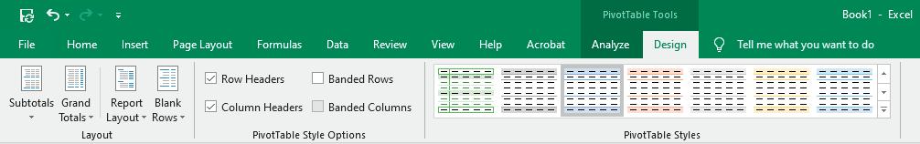
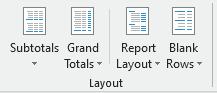
Figure 5.2. Layout options
Starting with the example of landfills, the uses of each of these functionalities are outlined below (see table 5.1).
Basic Concepts in Pivot Tables
ISBN: 978-84-18432-98-9
DOI: http://dx.doi.org/10.6035/Sapientia179
61
Beatriz Forés Julián, Alba Puig Denia, Rafael Lapiedra Alcamí, Francisco Fermín Mallén Broch, José Mª Fernández Yáñez
Table 5.1. Starting pivot table example
Sum of Kilograms Month
Landfill Product
1 2 3 4 5 6 Grand Total
Landfill 1 2500 2450 3200 3750 1800 1600 15300
Glass 900 800 700 1350 600 350 4700 Metal 400 500 800 600 400 400 3100 Paper and cardboard 300 450 700 450 300 350 2550
Plastic 600 500 600 900 400 300 3300 Textile 300 200 400 450 100 200 1650
Landfill 2 3200 2700 3200 4800 2150 1600 17650
Glass 500 600 700 750 400 300 3250 Metal 700 400 800 1050 300 150 3400
Paper and cardboard 800 800 700 1200 650 500 4650 Plastic 700 600 600 1050 500 450 3900 Textile 500 300 400 750 300 200 2450
Landfill 3 3000 3300 3200 4500 2700 1250 17950 Glass 700 800 600 1050 700 150 4000 Metal 600 400 300 900 300 250 2750
Paper and cardboard 1000 1100 1000 1500 900 400 5900 Plastic 500 700 900 750 600 350 3800 Textile 200 300 400 300 200 100 1500
Landfill 4 4000 3700 2500 6000 3000 2200 21400
Glass 800 900 300 1200 700 600 4500 Metal 900 700 500 1350 600 350 4400
Paper and cardboard 1500 1400 800 2250 1200 650 7800 Plastic 200 300 700 300 200 200 1900 Textile 600 400 200 900 300 400 2800 Landfill 5 4300 4300 4400 6450 4000 2300 25750
Glass 1300 1400 1200 1950 1300 750 7900 Metal 800 600 700 1200 500 450 4250
Paper and cardboard 700 800 1300 1050 700 600 5150 Plastic 1000 1100 400 1500 900 300 5200 Textile 500 400 800 750 600 200 3250
Grand Total 17000 16450 16500 25500 13650 8950 98050
5 .1 .1 . The Subtotals function
This function is used to show or hide subtotals in the pivot table, and means that the subtotals can be hidden, or shown at the top or bottom (see Figure 5.3).
62
Basic Concepts in Pivot Tables
ISBN: 978-84-18432-98-9
DOI: http://dx.doi.org/10.6035/Sapientia179
Beatriz Forés Julián, Alba Puig Denia, Rafael Lapiedra Alcamí, Francisco Fermín Mallén Broch, José Mª Fernández YáñezFigure 5.3. Subtotals function
Continuing with our example, when the Design , Do Not Show Subtotals option is selected, the subtotals do not appear for the landfills.
Table 5.2. Pivot table without subtotals
Sum of Kilograms Month
Landfill Product
Landfill 1
Landfill 2
Landfill 3
Landfill 4
Landfill 5
Grand Total
Basic Concepts in Pivot Tables

ISBN: 978-84-18432-98-9
1 2 3 4 5 6 Grand Total
Glass 900 800 700 1350 600 350 4700 Metal 400 500 800 600 400 400 3100
Paper and cardboard 300 450 700 450 300 350 2550 Plastic 600 500 600 900 400 300 3300 Textile 300 200 400 450 100 200 1650
Glass 500 600 700 750 400 300 3250 Metal 700 400 800 1050 300 150 3400
Paper and cardboard 800 800 700 1200 650 500 4650 Plastic 700 600 600 1050 500 450 3900 Textile 500 300 400 750 300 200 2450
Glass 700 800 600 1050 700 150 4000 Metal 600 400 300 900 300 250 2750
Paper and cardboard 1000 1100 1000 1500 900 400 5900 Plastic 500 700 900 750 600 350 3800 Textile 200 300 400 300 200 100 1500
Glass 800 900 300 1200 700 600 4500 Metal 900 700 500 1350 600 350 4400
Paper and cardboard 1500 1400 800 2250 1200 650 7800 Plastic 200 300 700 300 200 200 1900 Textile 600 400 200 900 300 400 2800
Glass 1300 1400 1200 1950 1300 750 7900 Metal 800 600 700 1200 500 450 4250
Paper and cardboard 700 800 1300 1050 700 600 5150 Plastic 1000 1100 400 1500 900 300 5200 Textile 500 400 800 750 600 200 3250
17000 16450 16500 25500 13650 8950 98050
63
DOI: http://dx.doi.org/10.6035/Sapientia179
Beatriz Forés Julián, Alba Puig Denia, Rafael Lapiedra Alcamí, Francisco Fermín Mallén Broch, José Mª Fernández YáñezOn the other hand, if the option chosen is Show all Subtotals at Bottom of Group , the subtotals of the number of kilos for each landfill will appear again (see Table 5.3).
Table 5.3. Pivot table with Show all Subtotals at Bottom of Group
Sum of Kilograms Month
Landfill Product 1 2 3 4 5 6 Grand Total
Landfill 1
Glass 900 800 700 1350 600 350 4700 Metal 400 500 800 600 400 400 3100 Paper and cardboard 300 450 700 450 300 350 2550 Plastic 600 500 600 900 400 300 3300 Textile 300 200 400 450 100 200 1650
Landfill 1 Total 2500 2450 3200 3750 1800 1600 15300
Landfill 2
Glass 500 600 700 750 400 300 3250 Metal 700 400 800 1050 300 150 3400 Paper and cardboard 800 800 700 1200 650 500 4650 Plastic 700 600 600 1050 500 450 3900 Textile 500 300 400 750 300 200 2450
Landfill 2 Total 3200 2700 3200 4800 2150 1600 17650
Landfill 3
Glass 700 800 600 1050 700 150 4000 Metal 600 400 300 900 300 250 2750 Paper and cardboard 1000 1100 1000 1500 900 400 5900 Plastic 500 700 900 750 600 350 3800 Textile 200 300 400 300 200 100 1500
Landfill 3 Total 3000 3300 3200 4500 2700 1250 17950
Landfill 4
Glass 800 900 300 1200 700 600 4500 Metal 900 700 500 1350 600 350 4400 Paper and cardboard 1500 1400 800 2250 1200 650 7800 Plastic 200 300 700 300 200 200 1900 Textile 600 400 200 900 300 400 2800
Landfill 4 Total 4000 3700 2500 6000 3000 2200 21400
Landfill 5
Glass 1300 1400 1200 1950 1300 750 7900 Metal 800 600 700 1200 500 450 4250 Paper and cardboard 700 800 1300 1050 700 600 5150 Plastic 1000 1100 400 1500 900 300 5200 Textile 500 400 800 750 600 200 3250
Landfill 5 Total 4300 4300 4400 6450 4000 2300 25750
Grand Total 17000 16450 16500 25500 13650 8950 98050
Finally, if you choose to Show all Subtotals at Top of Group , the result is similar to the previous option, but the location of the subtotals changes, as they now appear at the top, just before each location or province (see Table 5.4).
64
Basic Concepts in Pivot Tables
ISBN: 978-84-18432-98-9
DOI: http://dx.doi.org/10.6035/Sapientia179
Beatriz Forés Julián, Alba Puig Denia, Rafael Lapiedra Alcamí, Francisco Fermín Mallén Broch, José Mª Fernández YáñezTable 5.4. Pivot table with option Show all Subtotals at Bottom of Group
Sum of Kilograms Month
Landfill Product
1 2 3 4 5 6 Grand Total
Landfill 1 2500 2450 3200 3750 1800 1600 15300
Glass 900 800 700 1350 600 350 4700 Metal 400 500 800 600 400 400 3100
Paper and cardboard 300 450 700 450 300 350 2550 Plastic 600 500 600 900 400 300 3300 Textile 300 200 400 450 100 200 1650
Landfill 2 3200 2700 3200 4800 2150 1600 17650
Glass 500 600 700 750 400 300 3250 Metal 700 400 800 1050 300 150 3400
Paper and cardboard 800 800 700 1200 650 500 4650 Plastic 700 600 600 1050 500 450 3900 Textile 500 300 400 750 300 200 2450
Landfill 3 3000 3300 3200 4500 2700 1250 17950 Glass 700 800 600 1050 700 150 4000 Metal 600 400 300 900 300 250 2750
Paper and cardboard 1000 1100 1000 1500 900 400 5900 Plastic 500 700 900 750 600 350 3800 Textile 200 300 400 300 200 100 1500
Landfill 4 4000 3700 2500 6000 3000 2200 21400 Glass 800 900 300 1200 700 600 4500 Metal 900 700 500 1350 600 350 4400
Paper and cardboard 1500 1400 800 2250 1200 650 7800 Plastic 200 300 700 300 200 200 1900 Textile 600 400 200 900 300 400 2800
Landfill 5 4300 4300 4400 6450 4000 2300 25750 Glass 1300 1400 1200 1950 1300 750 7900 Metal 800 600 700 1200 500 450 4250 Paper and cardboard 700 800 1300 1050 700 600 5150 Plastic 1000 1100 400 1500 900 300 5200 Textile 500 400 800 750 600 200 3250
Grand Total 17000 16450 16500 25500 13650 8950 98050
Note:
If the tabular layout is chosen, rather than the compact or outline layout, the row showing all subtotals at the top is not available.
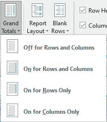
5 .1 .2 . Grand totals
As can be seen from its name, the Grand Totals symbol is used to show or hide the Grand Totals in the pivot table. This symbol provides four options (see Figure 5.4):
• Off for Rows and Columns.
• On for Rows and Columns.
• On for Rows only.
• On for Columns only.
Basic Concepts in Pivot Tables
ISBN: 978-84-18432-98-9
65
DOI: http://dx.doi.org/10.6035/Sapientia179
Beatriz Forés Julián, Alba Puig Denia, Rafael Lapiedra Alcamí, Francisco Fermín Mallén Broch, José Mª Fernández YáñezFigure 5.4. Grand totals
The result of applying each of these options to the example of a pivot table with the number of kilos per type of product is shown below (see Table 5.5).
Table 5.5. Initial pivot table example
Sum of Kilograms Month
Product
1 2 3 4 5 6 Grand Total
Glass 4200 4500 3500 6300 3700 2150 24350 Metal 3400 2600 3100 5100 2100 1600 17900 Paper and cardboard 4300 4550 4500 6450 3750 2500 26050 Plastic 3000 3200 3200 4500 2600 1600 18100 Textile 2100 1600 2200 3150 1500 1100 11650
Grand Total 17000 16450 16500 25500 13650 8950 98050
The Off for Rows and Columns option means that grand totals are not shown for either rows or columns (see Table 5.6).
66
Basic Concepts in Pivot Tables
ISBN: 978-84-18432-98-9
DOI: http://dx.doi.org/10.6035/Sapientia179
Beatriz Forés Julián, Alba Puig Denia, Rafael Lapiedra Alcamí, Francisco Fermín Mallén Broch, José Mª Fernández YáñezTable 5.6. Pivot table with grand totals Off for Rows and Columns
Sum of Kilograms Month
Product
1 2 3 4 5 6
Glass 4200 4500 3500 6300 3700 2150 Metal 3400 2600 3100 5100 2100 1600 Paper and cardboard 4300 4550 4500 6450 3750 2500 Plastic 3000 3200 3200 4500 2600 1600 Textile 2100 1600 2200 3150 1500 1100
The option On for Rows and Columns is used to show the grand totals for both rows and columns (see Table 5.7).
Table 5.7. Pivot table with grand totals On for Rows and Columns
Sum of Kilograms Month
Product
1 2 3 4 5 6 Grand Total
Glass 4200 4500 3500 6300 3700 2150 24350
Metal 3400 2600 3100 5100 2100 1600 17900 Paper and cardboard 4300 4550 4500 6450 3750 2500 26050 Plastic 3000 3200 3200 4500 2600 1600 18100 Textile 2100 1600 2200 3150 1500 1100 11650
Grand Total 17000 16450 16500 25500 13650 8950 98050
If you click on On for Rows Only , the totals will only appear in the rows (see Table 5.8).
Table 5.8. Pivot table with grand totals On for Rows Only
Sum of Kilograms Month
Product
1 2 3 4 5 6 Grand Total
Glass 4200 4500 3500 6300 3700 2150 24350 Metal 3400 2600 3100 5100 2100 1600 17900 Paper and cardboard 4300 4550 4500 6450 3750 2500 26050 Plastic 3000 3200 3200 4500 2600 1600 18100 Textile 2100 1600 2200 3150 1500 1100 11650
Finally, if On for Columns only is selected, Excel gives a table in which only the column totals appear (see Table 5.9).
67
Basic Concepts in Pivot Tables
ISBN: 978-84-18432-98-9
DOI: http://dx.doi.org/10.6035/Sapientia179
Beatriz Forés Julián, Alba Puig Denia, Rafael Lapiedra Alcamí, Francisco Fermín Mallén Broch, José Mª Fernández YáñezTable 5.9. Pivot table with grand totals On for Columns Only
Sum of Kilograms Month
Product
1 2 3 4 5 6
Glass 4200 4500 3500 6300 3700 2150 Metal 3400 2600 3100 5100 2100 1600
Paper and cardboard 4300 4550 4500 6450 3750 2500
Plastic 3000 3200 3200 4500 2600 1600
Textile 2100 1600 2200 3150 1500 1100
Grand Total 17000 16450 16500 25500 13650 8950
5 .1 .3 . The Report Layout function
The Report Layout function provides a choice between different ways of presenting the pivot table: in compact form, in outline form, in tabular form and repeating or not repeating the labels of the items (see Figure 5.5).

Figure 5.5. Options in Report Layout
Continuing with the example of landfills, the appearance of the pivot table if each of the options indicated were applied is shown below (see Tables 5.105.14).
Basic Concepts in Pivot Tables
ISBN: 978-84-18432-98-9
Beatriz
DOI: http://dx.doi.org/10.6035/Sapientia179
68
Forés Julián, Alba Puig Denia, Rafael Lapiedra Alcamí, Francisco Fermín Mallén Broch, José Mª Fernández Yáñez
Table 5.10. Show in Compact Form
Sum of Kilograms Column Labels
Row Labels
Landfill 1
1 2 3 4 5 6 Grand Total
2500 2450 3200 3750 1800 1600 15300
Glass 900 800 700 1350 600 350 4700 Metal 400 500 800 600 400 400 3100
Paper and cardboard 300 450 700 450 300 350 2550 Plastic 600 500 600 900 400 300 3300 Textile 300 200 400 450 100 200 1650 Landfill 2 3200 2700 3200 4800 2150 1600 17650
Glass 500 600 700 750 400 300 3250 Metal 700 400 800 1050 300 150 3400
Paper and cardboard 800 800 700 1200 650 500 4650 Plastic 700 600 600 1050 500 450 3900 Textile 500 300 400 750 300 200 2450 Landfill 3 3000 3300 3200 4500 2700 1250 17950
Glass 700 800 600 1050 700 150 4000 Metal 600 400 300 900 300 250 2750
Paper and cardboard 1000 1100 1000 1500 900 400 5900 Plastic 500 700 900 750 600 350 3800 Textile 200 300 400 300 200 100 1500 Landfill 4 4000 3700 2500 6000 3000 2200 21400
Glass 800 900 300 1200 700 600 4500 Metal 900 700 500 1350 600 350 4400 Paper and cardboard 1500 1400 800 2250 1200 650 7800 Plastic 200 300 700 300 200 200 1900 Textile 600 400 200 900 300 400 2800 Landfill 5 4300 4300 4400 6450 4000 2300 25750
Glass 1300 1400 1200 1950 1300 750 7900 Metal 800 600 700 1200 500 450 4250 Paper and cardboard 700 800 1300 1050 700 600 5150 Plastic 1000 1100 400 1500 900 300 5200 Textile 500 400 800 750 600 200 3250
Grand Total 17000 16450 16500 25500 13650 8950 98050
69
Basic Concepts in Pivot Tables
ISBN: 978-84-18432-98-9
DOI: http://dx.doi.org/10.6035/Sapientia179
Beatriz Forés Julián, Alba Puig Denia, Rafael Lapiedra Alcamí, Francisco Fermín Mallén Broch, José Mª Fernández YáñezTable 5.11. Show in Outline Form
Sum of Kilograms Month
Landfill Product
1 2 3 4 5 6 Grand Total
Landfill 1 2500 2450 3200 3750 1800 1600 15300
Glass 900 800 700 1350 600 350 4700
Metal 400 500 800 600 400 400 3100
Paper and cardboard 300 450 700 450 300 350 2550
Plastic 600 500 600 900 400 300 3300 Textile 300 200 400 450 100 200 1650
Landfill 2 3200 2700 3200 4800 2150 1600 17650
Glass 500 600 700 750 400 300 3250
Metal 700 400 800 1050 300 150 3400
Paper and cardboard 800 800 700 1200 650 500 4650
Plastic 700 600 600 1050 500 450 3900 Textile 500 300 400 750 300 200 2450
Landfill 3 3000 3300 3200 4500 2700 1250 17950
Glass 700 800 600 1050 700 150 4000 Metal 600 400 300 900 300 250 2750
Paper and cardboard 1000 1100 1000 1500 900 400 5900
Plastic 500 700 900 750 600 350 3800 Textile 200 300 400 300 200 100 1500
Landfill 4 4000 3700 2500 6000 3000 2200 21400
Glass 800 900 300 1200 700 600 4500 Metal 900 700 500 1350 600 350 4400
Paper and cardboard 1500 1400 800 2250 1200 650 7800 Plastic 200 300 700 300 200 200 1900 Textile 600 400 200 900 300 400 2800
Landfill 5 4300 4300 4400 6450 4000 2300 25750
Glass 1300 1400 1200 1950 1300 750 7900 Metal 800 600 700 1200 500 450 4250
Paper and cardboard 700 800 1300 1050 700 600 5150 Plastic 1000 1100 400 1500 900 300 5200 Textile 500 400 800 750 600 200 3250
Grand Total 17000 16450 16500 25500 13650 8950 98050
70
Basic Concepts in Pivot Tables
ISBN: 978-84-18432-98-9
DOI: http://dx.doi.org/10.6035/Sapientia179
Beatriz Forés Julián, Alba Puig Denia, Rafael Lapiedra Alcamí, Francisco Fermín Mallén Broch, José Mª Fernández YáñezTable 5.12. Show in Tabular Form
Sum of Kilograms Month
Landfill Product 1 2 3 4 5 6 Grand Total
Landfill 1 Glass 900 800 700 1350 600 350 4700
Metal 400 500 800 600 400 400 3100
Paper and cardboard 300 450 700 450 300 350 2550 Plastic 600 500 600 900 400 300 3300 Textile 300 200 400 450 100 200 1650
Landfill 1 Total 2500 2450 3200 3750 1800 1600 15300
Landfill 2 Glass 500 600 700 750 400 300 3250
Metal 700 400 800 1050 300 150 3400
Paper and cardboard 800 800 700 1200 650 500 4650
Plastic 700 600 600 1050 500 450 3900 Textile 500 300 400 750 300 200 2450
Landfill 2 Total 3200 2700 3200 4800 2150 1600 17650
Landfill 3 Glass 700 800 600 1050 700 150 4000 Metal 600 400 300 900 300 250 2750
Paper and cardboard 1000 1100 1000 1500 900 400 5900
Plastic 500 700 900 750 600 350 3800 Textile 200 300 400 300 200 100 1500
Landfill 3 Total 3000 3300 3200 4500 2700 1250 17950
Landfill 4 Glass 800 900 300 1200 700 600 4500 Metal 900 700 500 1350 600 350 4400
Paper and cardboard 1500 1400 800 2250 1200 650 7800 Plastic 200 300 700 300 200 200 1900 Textile 600 400 200 900 300 400 2800
Landfill 4 Total 4000 3700 2500 6000 3000 2200 21400
Landfill 5 Glass 1300 1400 1200 1950 1300 750 7900
Metal 800 600 700 1200 500 450 4250
Paper and cardboard 700 800 1300 1050 700 600 5150 Plastic 1000 1100 400 1500 900 300 5200 Textile 500 400 800 750 600 200 3250
Landfill 5 Total 4300 4300 4400 6450 4000 2300 25750
Grand Total 17000 16450 16500 25500 13650 8950 98050
71
Basic Concepts in Pivot Tables
ISBN: 978-84-18432-98-9
Beatriz
DOI: http://dx.doi.org/10.6035/Sapientia179
Forés Julián, Alba Puig Denia, Rafael Lapiedra Alcamí, Francisco Fermín Mallén Broch, José Mª Fernández YáñezSum of Kilograms
Table 5.13. Repeat All Item Labels
Month
Landfill Product 1 2 3 4 5 6 Grand Total
Landfill 1 2500 2450 3200 3750 1800 1600 15300
Landfill 1 Glass 900 800 700 1350 600 350 4700
Landfill 1 Metal 400 500 800 600 400 400 3100
Landfill 1 Paper and cardboard 300 450 700 450 300 350 2550
Landfill 1 Plastic 600 500 600 900 400 300 3300
Landfill 1 Textile 300 200 400 450 100 200 1650
Landfill 2 3200 2700 3200 4800 2150 1600 17650
Landfill 2 Glass 500 600 700 750 400 300 3250
Landfill 2 Metal 700 400 800 1050 300 150 3400
Landfill 2 Paper and cardboard 800 800 700 1200 650 500 4650 Landfill 2 Plastic 700 600 600 1050 500 450 3900 Landfill 2 Textile 500 300 400 750 300 200 2450
Landfill 3 3000 3300 3200 4500 2700 1250 17950
Landfill 3 Glass 700 800 600 1050 700 150 4000
Landfill 3 Metal 600 400 300 900 300 250 2750
Landfill 3 Paper and cardboard 1000 1100 1000 1500 900 400 5900
Landfill 3 Plastic 500 700 900 750 600 350 3800
Landfill 3 Textile 200 300 400 300 200 100 1500
Landfill 4 4000 3700 2500 6000 3000 2200 21400
Landfill 4 Glass 800 900 300 1200 700 600 4500
Landfill 4 Metal 900 700 500 1350 600 350 4400
Landfill 4 Paper and cardboard 1500 1400 800 2250 1200 650 7800
Landfill 4 Plastic 200 300 700 300 200 200 1900
Landfill 4 Textile 600 400 200 900 300 400 2800
Landfill 5 4300 4300 4400 6450 4000 2300 25750
Landfill 5 Glass 1300 1400 1200 1950 1300 750 7900
Landfill 5 Metal 800 600 700 1200 500 450 4250
Landfill 5 Paper and cardboard 700 800 1300 1050 700 600 5150
Landfill 5 Plastic 1000 1100 400 1500 900 300 5200
Landfill 5 Textile 500 400 800 750 600 200 3250
Grand Total 17000 16450 16500 25500 13650 8950 98050
72
Basic Concepts in Pivot Tables
ISBN: 978-84-18432-98-9
Beatriz Forés Julián, Alba Puig Denia, Rafael Lapiedra Alcamí, Francisco Fermín Mallén Broch, José Mª Fernández Yáñez DOI: http://dx.doi.org/10.6035/Sapientia179
Sum of Kilograms
Landfill Product
Table 5.14. Do Not Repeat Item Labels
Month
1 2 3 4 5 6 Grand Total
Landfill 1 2500 2450 3200 3750 1800 1600 15300
Glass 900 800 700 1350 600 350 4700
Metal 400 500 800 600 400 400 3100
Paper and cardboard 300 450 700 450 300 350 2550
Plastic 600 500 600 900 400 300 3300 Textile 300 200 400 450 100 200 1650
Landfill 2 3200 2700 3200 4800 2150 1600 17650
Glass 500 600 700 750 400 300 3250
Metal 700 400 800 1050 300 150 3400
Paper and cardboard 800 800 700 1200 650 500 4650
Plastic 700 600 600 1050 500 450 3900 Textile 500 300 400 750 300 200 2450
Landfill 3 3000 3300 3200 4500 2700 1250 17950
Glass 700 800 600 1050 700 150 4000 Metal 600 400 300 900 300 250 2750
Paper and cardboard 1000 1100 1000 1500 900 400 5900
Plastic 500 700 900 750 600 350 3800
Textile 200 300 400 300 200 100 1500
Landfill 4 4000 3700 2500 6000 3000 2200 21400
Glass 800 900 300 1200 700 600 4500
Metal 900 700 500 1350 600 350 4400
Paper and cardboard 1500 1400 800 2250 1200 650 7800 Plastic 200 300 700 300 200 200 1900 Textile 600 400 200 900 300 400 2800
Landfill 5 4300 4300 4400 6450 4000 2300 25750
Glass 1300 1400 1200 1950 1300 750 7900
Metal 800 600 700 1200 500 450 4250
Paper and cardboard 700 800 1300 1050 700 600 5150
Plastic 1000 1100 400 1500 900 300 5200 Textile 500 400 800 750 600 200 3250
Grand Total 17000 16450 16500 25500 13650 8950 98050
5 .1 .4 . Blank rows
This option is used to insert a blank row between each grouped item in the pivot table. Once the row is inserted, there is also the option to return to the initial situation (see Figure 5.6).
73
Basic Concepts in Pivot Tables
ISBN: 978-84-18432-98-9
DOI: http://dx.doi.org/10.6035/Sapientia179
Beatriz Forés Julián, Alba Puig Denia, Rafael Lapiedra Alcamí, Francisco Fermín Mallén Broch, José Mª Fernández YáñezFigure 5.6. Insert Blank Rows
If the option Insert Blank Lines after Each Item is activated, the result would be as shown in Table 5.15 below.
Table 5.15. Example of Blank Lines after Each Item in the landfills example
Sum of Kilograms Month
Landfill Product
1 2 3 4 5 6 Grand Total
Landfill 1 2500 2450 3200 3750 1800 1600 15300
Glass 900 800 700 1350 600 350 4700
Metal 400 500 800 600 400 400 3100
Paper and cardboard 300 450 700 450 300 350 2550 Plastic 600 500 600 900 400 300 3300 Textile 300 200 400 450 100 200 1650
Landfill 2 3200 2700 3200 4800 2150 1600 17650
Glass 500 600 700 750 400 300 3250
Metal 700 400 800 1050 300 150 3400 Paper and cardboard 800 800 700 1200 650 500 4650 Plastic 700 600 600 1050 500 450 3900 Textile 500 300 400 750 300 200 2450
Landfill 3 3000 3300 3200 4500 2700 1250 17950
Glass 700 800 600 1050 700 150 4000 Metal 600 400 300 900 300 250 2750
Paper and cardboard 1000 1100 1000 1500 900 400 5900 Plastic 500 700 900 750 600 350 3800 Textile 200 300 400 300 200 100 1500
Landfill 4
4000 3700 2500 6000 3000 2200 21400
Glass 800 900 300 1200 700 600 4500
Metal 900 700 500 1350 600 350 4400
Paper and cardboard 1500 1400 800 2250 1200 650 7800 Plastic 200 300 700 300 200 200 1900 Textile 600 400 200 900 300 400 2800
Landfill 5
4300 4300 4400 6450 4000 2300 25750
Glass 1300 1400 1200 1950 1300 750 7900
Metal 800 600 700 1200 500 450 4250
Paper and cardboard 700 800 1300 1050 700 600 5150
Plastic 1000 1100 400 1500 900 300 5200 Textile 500 400 800 750 600 200 3250
Grand Total 17000 16450 16500 25500 13650 8950 98050
74
Basic Concepts in Pivot Tables

ISBN: 978-84-18432-98-9
DOI: http://dx.doi.org/10.6035/Sapientia179
Beatriz Forés Julián, Alba Puig Denia, Rafael Lapiedra Alcamí, Francisco Fermín Mallén Broch, José Mª Fernández YáñezIf the Remove Blank Line after Each Item option is selected, it will return to the starting point where there is no blank line.
5 .2 . PIVOT TABLE STYLE OPTIONS

The available set of pivot table style options is designed to make the data summarized in the table easier to read, by highlighting different parts of the table using bold text or shading. There are four options that can be enabled simultaneously or separately (see Figure 5.7).
Figure 5.7. Pivot Table Style Options
Continuing with the example used in previous sections, tables 5.16-5.20 below show the results of applying each of these options.
75
Basic Concepts in Pivot Tables
ISBN: 978-84-18432-98-9
DOI: http://dx.doi.org/10.6035/Sapientia179
Beatriz Forés Julián, Alba Puig Denia, Rafael Lapiedra Alcamí, Francisco Fermín Mallén Broch, José Mª Fernández YáñezTable 5.16. Row Headers
Sum of Kilograms Month
Landfill Product 1 2 3 4 5 6 Grand Total
Landfill 1 2500 2450 3200 3750 1800 1600 15300
Glass 900 800 700 1350 600 350 4700
Metal 400 500 800 600 400 400 3100
Paper and cardboard 300 450 700 450 300 350 2550
Plastic 600 500 600 900 400 300 3300 Textile 300 200 400 450 100 200 1650
Landfill 2 3200 2700 3200 4800 2150 1600 17650
Glass 500 600 700 750 400 300 3250
Metal 700 400 800 1050 300 150 3400
Paper and cardboard 800 800 700 1200 650 500 4650
Plastic 700 600 600 1050 500 450 3900 Textile 500 300 400 750 300 200 2450
Landfill 3 3000 3300 3200 4500 2700 1250 17950
Glass 700 800 600 1050 700 150 4000 Metal 600 400 300 900 300 250 2750
Paper and cardboard 1000 1100 1000 1500 900 400 5900
Plastic 500 700 900 750 600 350 3800
Textile 200 300 400 300 200 100 1500
Landfill 4 4000 3700 2500 6000 3000 2200 21400
Glass 800 900 300 1200 700 600 4500
Metal 900 700 500 1350 600 350 4400
Paper and cardboard 1500 1400 800 2250 1200 650 7800
Plastic 200 300 700 300 200 200 1900 Textile 600 400 200 900 300 400 2800
Landfill 5 4300 4300 4400 6450 4000 2300 25750
Glass 1300 1400 1200 1950 1300 750 7900
Metal 800 600 700 1200 500 450 4250
Paper and cardboard 700 800 1300 1050 700 600 5150
Plastic 1000 1100 400 1500 900 300 5200 Textile 500 400 800 750 600 200 3250
Grand Total 17000 16450 16500 25500 13650 8950 98050
The table changes when the Row Headers option is enabled and disabled.
76
Basic Concepts in Pivot Tables
ISBN: 978-84-18432-98-9
Beatriz
DOI: http://dx.doi.org/10.6035/Sapientia179
Forés Julián, Alba Puig Denia, Rafael Lapiedra Alcamí, Francisco Fermín Mallén Broch, José Mª Fernández YáñezTable 5.17. Column Headers
Sum of Kilograms Month
Landfill Product
Landfill 1
1 2 3 4 5 6 Grand Total
Glass 900 800 700 1350 600 350 4700
Metal 400 500 800 600 400 400 3100
Paper and cardboard 300 450 700 450 300 350 2550
Plastic 600 500 600 900 400 300 3300 Textile 300 200 400 450 100 200 1650
Landfill 1 Total 2500 2450 3200 3750 1800 1600 15300
Landfill 2
Glass 500 600 700 750 400 300 3250
Metal 700 400 800 1050 300 150 3400
Paper and cardboard 800 800 700 1200 650 500 4650 Plastic 700 600 600 1050 500 450 3900 Textile 500 300 400 750 300 200 2450
Landfill 2 Total 3200 2700 3200 4800 2150 1600 17650
Landfill 3
Glass 700 800 600 1050 700 150 4000 Metal 600 400 300 900 300 250 2750
Paper and cardboard 1000 1100 1000 1500 900 400 5900
Plastic 500 700 900 750 600 350 3800 Textile 200 300 400 300 200 100 1500
Landfill 3 Total 3000 3300 3200 4500 2700 1250 17950
Landfill 4
Glass 800 900 300 1200 700 600 4500
Metal 900 700 500 1350 600 350 4400
Paper and cardboard 1500 1400 800 2250 1200 650 7800 Plastic 200 300 700 300 200 200 1900 Textile 600 400 200 900 300 400 2800
Landfill 4 Total 4000 3700 2500 6000 3000 2200 21400
Landfill 5
Glass 1300 1400 1200 1950 1300 750 7900 Metal 800 600 700 1200 500 450 4250 Paper and cardboard 700 800 1300 1050 700 600 5150 Plastic 1000 1100 400 1500 900 300 5200 Textile 500 400 800 750 600 200 3250
Landfill 5 Total 4300 4300 4400 6450 4000 2300 25750
Grand Total 17000 16450 16500 25500 13650 8950 98050
When the Column Headers option is enabled , the first row of the table where the headings or names of each column are located is highlighted.
77
Basic Concepts in Pivot Tables
ISBN: 978-84-18432-98-9
DOI: http://dx.doi.org/10.6035/Sapientia179
Beatriz Forés Julián, Alba Puig Denia, Rafael Lapiedra Alcamí, Francisco Fermín Mallén Broch, José Mª Fernández YáñezSum of Kilograms
Table 5.18. Banded Rows
Month
Landfill Product 1 2 3 4 5 6 Grand Total
Landfill 1
Glass 900 800 700 1350 600 350 4700
Metal 400 500 800 600 400 400 3100
Paper and cardboard 300 450 700 450 300 350 2550 Plastic 600 500 600 900 400 300 3300 Textile 300 200 400 450 100 200 1650
Landfill 1 Total 2500 2450 3200 3750 1800 1600 15300
Landfill 2
Glass 500 600 700 750 400 300 3250
Metal 700 400 800 1050 300 150 3400
Paper and cardboard 800 800 700 1200 650 500 4650 Plastic 700 600 600 1050 500 450 3900 Textile 500 300 400 750 300 200 2450
Landfill 2 Total 3200 2700 3200 4800 2150 1600 17650
Landfill 3
Glass 700 800 600 1050 700 150 4000 Metal 600 400 300 900 300 250 2750
Paper and cardboard 1000 1100 1000 1500 900 400 5900
Plastic 500 700 900 750 600 350 3800 Textile 200 300 400 300 200 100 1500
Landfill 3 Total 3000 3300 3200 4500 2700 1250 17950
Landfill 4
Glass 800 900 300 1200 700 600 4500 Metal 900 700 500 1350 600 350 4400
Paper and cardboard 1500 1400 800 2250 1200 650 7800 Plastic 200 300 700 300 200 200 1900 Textile 600 400 200 900 300 400 2800
Landfill 4 Total 4000 3700 2500 6000 3000 2200 21400
Landfill 5
Glass 1300 1400 1200 1950 1300 750 7900 Metal 800 600 700 1200 500 450 4250 Paper and cardboard 700 800 1300 1050 700 600 5150 Plastic 1000 1100 400 1500 900 300 5200 Textile 500 400 800 750 600 200 3250
Landfill 5 Total 4300 4300 4400 6450 4000 2300 25750
Grand Total 17000 16450 16500 25500 13650 8950 98050
Using the Banded Rows option, some rows are alternately shaded, so that even rows appear in a different format to odd ones.
78
Basic Concepts in Pivot Tables
ISBN: 978-84-18432-98-9
Beatriz Forés Julián, Alba Puig Denia, Rafael Lapiedra Alcamí, Francisco Fermín Mallén Broch, José Mª Fernández Yáñez
DOI: http://dx.doi.org/10.6035/Sapientia179
Table 5.19. Banded Columns
Sum of Kilograms Month
Landfill Product 1 2 3 4 5 6 Grand Total
Landfill 1
Glass 900 800 700 1350 600 350 4700
Metal 400 500 800 600 400 400 3100
Paper and cardboard 300 450 700 450 300 350 2550 Plastic 600 500 600 900 400 300 3300 Textile 300 200 400 450 100 200 1650
Landfill 1 Total 2500 2450 3200 3750 1800 1600 15300
Landfill 2
Glass 500 600 700 750 400 300 3250
Metal 700 400 800 1050 300 150 3400
Paper and cardboard 800 800 700 1200 650 500 4650 Plastic 700 600 600 1050 500 450 3900 Textile 500 300 400 750 300 200 2450
Landfill 2 Total 3200 2700 3200 4800 2150 1600 17650
Landfill 3
Glass 700 800 600 1050 700 150 4000 Metal 600 400 300 900 300 250 2750
Paper and cardboard 1000 1100 1000 1500 900 400 5900 Plastic 500 700 900 750 600 350 3800 Textile 200 300 400 300 200 100 1500
Landfill 3 Total 3000 3300 3200 4500 2700 1250 17950
Landfill 4
Glass 800 900 300 1200 700 600 4500 Metal 900 700 500 1350 600 350 4400
Paper and cardboard 1500 1400 800 2250 1200 650 7800 Plastic 200 300 700 300 200 200 1900 Textile 600 400 200 900 300 400 2800
Landfill 4 Total 4000 3700 2500 6000 3000 2200 21400
Landfill 5
Glass 1300 1400 1200 1950 1300 750 7900 Metal 800 600 700 1200 500 450 4250 Paper and cardboard 700 800 1300 1050 700 600 5150 Plastic 1000 1100 400 1500 900 300 5200 Textile 500 400 800 750 600 200 3250
Landfill 5 Total 4300 4300 4400 6450 4000 2300 25750
Grand Total 17000 16450 16500 25500 13650 8950 98050
In a similar way to the Banded Rows option, this time the shading appears in some columns, creating a presentation where one column with shading and another without shading alternate. Both this option and the one above are useful when the pivot table contains a lot of data, since it makes reading easier. Finally, Table 5.20 shows an example of a table with all the options above enabled.
79
Basic Concepts in Pivot Tables
ISBN: 978-84-18432-98-9
Beatriz Forés Julián, Alba Puig Denia, Rafael Lapiedra Alcamí, Francisco Fermín Mallén Broch, José Mª Fernández Yáñez
DOI: http://dx.doi.org/10.6035/Sapientia179
Table 5.20. Example with all Pivot Table Style Options enabled
Sum of Kilograms
Month
Landfill Product 1 2 3 4 5 6 Grand Total
Landfill 1
Glass 900 800 700 1350 600 350 4700 Metal 400 500 800 600 400 400 3100 Paper and cardboard 300 450 700 450 300 350 2550 Plastic 600 500 600 900 400 300 3300 Textile 300 200 400 450 100 200 1650
Landfill 1 Total 2500 2450 3200 3750 1800 1600 15300
Landfill 2
Glass 500 600 700 750 400 300 3250 Metal 700 400 800 1050 300 150 3400
Paper and cardboard 800 800 700 1200 650 500 4650 Plastic 700 600 600 1050 500 450 3900 Textile 500 300 400 750 300 200 2450
Landfill 2 Total 3200 2700 3200 4800 2150 1600 17650
Landfill 3
Glass 700 800 600 1050 700 150 4000 Metal 600 400 300 900 300 250 2750 Paper and cardboard 1000 1100 1000 1500 900 400 5900 Plastic 500 700 900 750 600 350 3800 Textile 200 300 400 300 200 100 1500
Landfill 3 Total 3000 3300 3200 4500 2700 1250 17950
Landfill 4
Glass 800 900 300 1200 700 600 4500 Metal 900 700 500 1350 600 350 4400
Paper and cardboard 1500 1400 800 2250 1200 650 7800 Plastic 200 300 700 300 200 200 1900 Textile 600 400 200 900 300 400 2800
Landfill 4 Total 4000 3700 2500 6000 3000 2200 21400
Landfill 5
Glass 1300 1400 1200 1950 1300 750 7900 Metal 800 600 700 1200 500 450 4250 Paper and cardboard 700 800 1300 1050 700 600 5150 Plastic 1000 1100 400 1500 900 300 5200 Textile 500 400 800 750 600 200 3250
Landfill 5 Total 4300 4300 4400 6450 4000 2300 25750
Grand Total 17000 16450 16500 25500 13650 8950 98050
5 .3 . PIVOT TABLE STYLES
Various predefined styles can be applied to a pivot table using this option, which is a quick way to improve the presentation of the table. It is possible to choose between different intensities of colours or present the rows or columns with bands (see Figure 5.8).
80
Basic Concepts in Pivot Tables
ISBN: 978-84-18432-98-9
Beatriz Forés Julián, Alba Puig Denia, Rafael Lapiedra Alcamí, Francisco Fermín Mallén Broch, José Mª Fernández Yáñez DOI: http://dx.doi.org/10.6035/Sapientia179
Figure 5.8. Pivot table styles
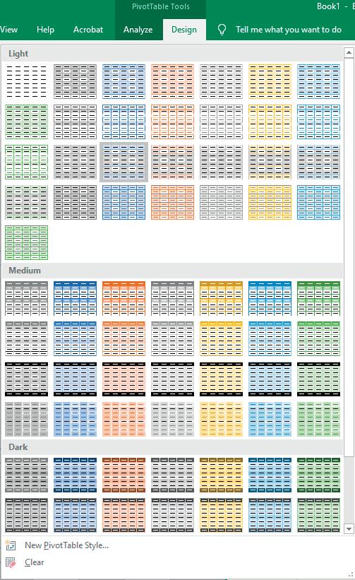
Although these styles are limited, it is also possible to create new custom styles using the New Pivot Table Style option (see Figure 5.9). These self-made styles can be saved as templates. Finally, the Clear option is used to remove the styles applied to a pivot table.
Basic Concepts in Pivot Tables
ISBN: 978-84-18432-98-9
DOI: http://dx.doi.org/10.6035/Sapientia179
81
Beatriz Forés Julián, Alba Puig Denia, Rafael Lapiedra Alcamí, Francisco Fermín Mallén Broch, José Mª Fernández Yáñez
Basic Concepts in Pivot Tables
ISBN: 978-84-18432-98-9
Figure 5.9. Custom Pivot Table Style
DOI: http://dx.doi.org/10.6035/Sapientia179

82
Beatriz Forés Julián, Alba Puig Denia, Rafael Lapiedra Alcamí, Francisco Fermín Mallén Broch, José Mª Fernández Yáñez
Chapter 6: Applying conditional formats
The Home tab can be used to access the Conditional Formatting option (see Figure 6.1).
Figure 6.1. Conditional Formatting
This option is not exclusive to pivot tables, but is applicable in any other type of tables. However, the combination of conditional formatting functionalities with pivot tables can be very useful.
Dynamic tables are often made up of numerous data, and it may be interesting to determine any changes in them. Using a type of indicator may be useful for this purpose. In some cases, it may be interesting to know how a variable evolves over time, whether it has increased or decreased, or simply how it has evolved in relation to an ideal value.
The example of waste collection will be used for this chapter. We generate a pivot table that summarizes the kilograms of each type of recycled product collected in each quarter (see Table 6.1).
Basic Concepts in Pivot Tables
ISBN: 978-84-18432-98-9
DOI: http://dx.doi.org/10.6035/Sapientia179
83
Beatriz Forés Julián, Alba Puig Denia, Rafael Lapiedra Alcamí, Francisco Fermín Mallén Broch, José Mª Fernández Yáñez
Table 6.1. Starting pivot table example
Sum of Kilograms Quarter
Product Quarter 1 Quarter 2 Grand Total
Glass 12200 12150 24350 Metal 9100 8800 17900 Paper and cardboard 13350 12700 26050 Plastic 9400 8700 18100 Textile 5900 5750 11650 Grand Total 49950 48100 98050
A comparison of the data shows that the amounts of waste collected during the first quarter are higher than those in the second. However, another view of the table could facilitate analysis of the data (see Table 6.2).
Table 6.2. Pivot table with conditional formatting
Sum of Kilograms Quarter
Product Quarter 1 Quarter 2 Grand Total
Glass 12200 12150 24350 Metal 9100 8800 17900 Paper and cardboard 13350 12700 26050 Plastic 9400 8700 18100 Textile 5900 5750 11650 Grand Total 49950 48100 98050
Colours of varying intensities could also be used to reflect whether or not the quantities meet a certain objective. Let us suppose that the collection of quantities greater than 10,000 kg is considered adequate for each type of product. By contrast, amounts lower than this amount would imply that there is still room for improvement. In Table 6.3 below, a darker colour is associated with when the collected quantities are not acceptable, and a lighter colour with when they are.
84
Basic Concepts in Pivot Tables
ISBN: 978-84-18432-98-9
DOI: http://dx.doi.org/10.6035/Sapientia179
Beatriz Forés Julián, Alba Puig Denia, Rafael Lapiedra Alcamí, Francisco Fermín Mallén Broch, José Mª Fernández YáñezSum
Table 6.3. Pivot table with conditional formatting linked to colour
The interpretation of the data could be even more complex if we include more data in our table, as could be the case if we are interested in distinguishing between the amounts collected each month or in different landfills.
In this case, it is advisable to use conditional formats in the pivot table. These formats are very flexible, and provide many possibilities. As a result, only some of them will be explained below.
The Conditional Formatting option is on the Home tab, and it is possible to choose from the possibilities shown in Figure 6.2.
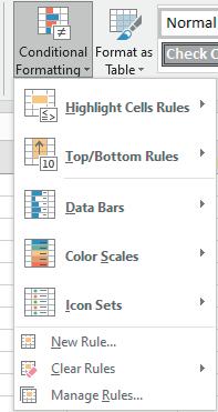
Basic Concepts in Pivot Tables
ISBN: 978-84-18432-98-9
Figure 6.2. Content of the Conditional Formatting option
85
Beatriz Forés Julián, Alba Puig Denia, Rafael Lapiedra Alcamí, Francisco Fermín Mallén Broch, José Mª Fernández Yáñez DOI: http://dx.doi.org/10.6035/Sapientia179
Quarter
Quarter
Grand
12200 12150
Metal
Paper
13350
Plastic
Textile
of Kilograms Quarter Product
1
2
Total Glass
24350
9100 8800 17900
and cardboard
12700 26050
9400 8700 18100
5900 5750 11650 Grand Total 49950 48100 98050
6 .1 . HIGHLIGHT CELLS RULES
Cells rules highlight data in the pivot table that meet a certain condition (see Figure 6.3). For example, if the data are numbers, it is possible to highlight those that are higher or lower than a certain amount. It is also possible to highlight cells that contain specific text or dates.
Figure 6.3. Content of Highlight Cells Rules option
Returning to the example of waste collection, suppose that we want to know in which quarter the collection of each product was greater than 10,000 kilos. The first step is to select the data range in which we want to apply conditional formatting.
By following the sequence Conditional Formatting , Highlight Cells Rules , Greater than , a dialog box appears that must be completed with the amount we want to specify (in this case 10,000) (see Figure 6.4). A predetermined format to apply to those cells also appears by default, but it could be changed for other predefined options or even completely customized with a desired format for cells that meet the specified condition.
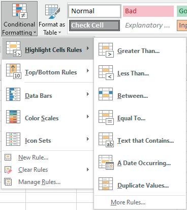
Basic Concepts in Pivot Tables
ISBN: 978-84-18432-98-9
DOI: http://dx.doi.org/10.6035/Sapientia179
86
Beatriz Forés Julián, Alba Puig Denia, Rafael Lapiedra Alcamí, Francisco Fermín Mallén Broch, José Mª Fernández Yáñez
The
Basic Concepts in Pivot Tables
ISBN: 978-84-18432-98-9

87
Forés Julián, Alba Puig Denia, Rafael Lapiedra Alcamí, Francisco Fermín Mallén Broch, José
Beatriz
Mª Fernández Yáñez DOI: http://dx.doi.org/10.6035/Sapientia179
Result of conditional formatting Sum of Kilograms Quarter Product Quarter 1 Quarter 2 Grand Total Glass 12200 12150 24350 Metal 9100 8800 17900 Paper and cardboard 13350 12700 26050 Plastic 9400 8700 18100 Textile 5900 5750 11650 Grand Total 49950 48100 98050
result is shown in Table 6.4 below. Table 6.4.
It is also possible to create new rules using the Conditional Formatting, Highlight Cells Rules, More Rules option for different cell selections (see Figure 6.5).
Figure 6.5. New Formatting Rule
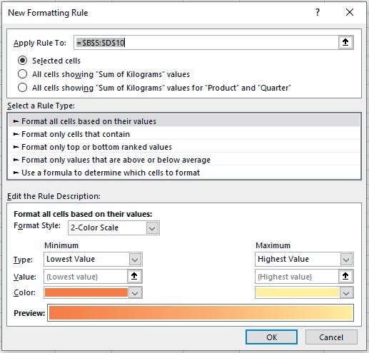
Figures 6.6 to 6.12 below present the different Highlight Cells Rules options.

Basic Concepts in Pivot Tables
ISBN: 978-84-18432-98-9
Figure 6.6. Format cells that are Greater than
DOI: http://dx.doi.org/10.6035/Sapientia179
88
Beatriz Forés Julián, Alba Puig Denia, Rafael Lapiedra Alcamí, Francisco Fermín Mallén Broch, José Mª Fernández Yáñez
Figure 6.7. Format cells that are Less than
Figure 6.8. Format cells that are Between
Figure 6.9. Format cells that are Equal to
Figure 6.10. Format cells that contain text with a specified string of letters
89
Basic Concepts in Pivot Tables


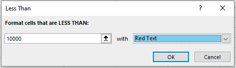
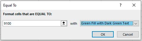
ISBN: 978-84-18432-98-9
DOI: http://dx.doi.org/10.6035/Sapientia179
Beatriz Forés Julián, Alba Puig Denia, Rafael Lapiedra Alcamí, Francisco Fermín Mallén Broch, José Mª Fernández YáñezThis option, as well as the next two, is only available for non-value fields.

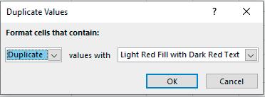
Figure 6.11. Format cells that contain A Date
Figure 6.12. Format cells that contain Duplicate Values
6 .2 . TOP/BOTTOM RULES
This time, suppose that we want to highlight only the highest or lowest values (see Figure 6.13). We must specify exactly how many values we want to highlight, e.g. if we want to apply conditional formatting to the 10 highest values, or to the highest 10%. It might also be useful to highlight the lowest 10 values or the lowest 10%. Another option would be to apply the format to cells that are above or below the average value.
90
Basic Concepts in Pivot Tables
ISBN: 978-84-18432-98-9
DOI: http://dx.doi.org/10.6035/Sapientia179
Beatriz Forés Julián, Alba Puig Denia, Rafael Lapiedra Alcamí, Francisco Fermín Mallén Broch, José Mª Fernández YáñezFigure 6.13. Top/Bottom rules
Returning to the table containing the amounts of each type of waste collected in each quarter, the data for each quarter must be selected with the mouse (see Table 6.5).
Table 6.5. Selection of the data range to analyze
91
Basic Concepts in Pivot Tables

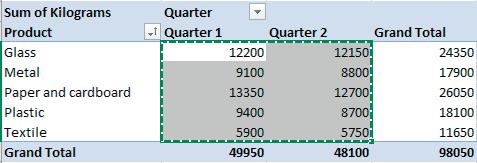
ISBN: 978-84-18432-98-9
DOI: http://dx.doi.org/10.6035/Sapientia179
Beatriz Forés Julián, Alba Puig Denia, Rafael Lapiedra Alcamí, Francisco Fermín Mallén Broch, José Mª Fernández YáñezIf we want to highlight the 3 highest values in dark green, the following steps are required: Conditional Formatting , Top/Bottom Rules , Top 10 Items . In the dialog box that appears, 10 must be replaced by 3 (since we only want the three highest values in our selection) (see Figure 6.14).
Sum of Kilograms Quarter
Product Quarter 1 Quarter 2 Grand Total Glass 12200 12150 24350 Metal 9100 8800 17900 Paper and cardboard 13350 12700 26050 Plastic 9400 8700 18100 Textile 5900 5750 11650 Grand Total 49950 48100 98050
Figure 6.14. Conditional formatting with the 3 highest values
On the other hand, if the “Top 10%” option is chosen and the number 10 is kept in the dialog box, only one value would be highlighted (we have 10 values, so 10% of the best is 1) (see Figure 6.15).

92
Basic Concepts in Pivot Tables
ISBN: 978-84-18432-98-9
Beatriz
DOI: http://dx.doi.org/10.6035/Sapientia179
Forés Julián, Alba Puig Denia, Rafael Lapiedra Alcamí, Francisco Fermín Mallén Broch, José Mª Fernández YáñezFigure 6.15. Conditional formatting with the highest 10% of values
6 .3 . DATA BARS
This option combines the utility of viewing the table with the data and a graph at the same time (see Figure 6.16). This is because a colour bar can be included in each cell with this option. This bar represents the value of the cell, and the width will vary depending on the magnitude of the value contained in each cell. It is also possible to choose between a solid or gradient fill for the bars.
Basic Concepts in Pivot Tables
ISBN: 978-84-18432-98-9

93
Quarter Product Quarter
Quarter
Grand Total
Beatriz Forés Julián, Alba Puig Denia, Rafael Lapiedra Alcamí, Francisco Fermín Mallén Broch, José Mª Fernández Yáñez DOI: http://dx.doi.org/10.6035/Sapientia179 Sum of Kilograms
1
2
Glass 12200 12150 24350 Metal 9100 8800 17900 Paper and cardboard 13350 12700 26050 Plastic 9400 8700 18100 Textile 5900 5750 11650 Grand Total 49950 48100 98050
Figure 6.16. Data Bars
For example, in order to generate data bars in green in our example (see Table 6.6-6.7), we need to select the data, follow the instruction Conditional Formatting , Data Bars and finally, select the colour we want to use, as well as whether it is weathered or solid.

Table 6.6. Starting pivot table example
Sum of Kilograms Quarter
Product Quarter 1 Quarter 2 Grand Total
Glass 12200 12150 24350 Metal 9100 8800 17900 Paper and cardboard 13350 12700 26050 Plastic 9400 8700 18100 Textile 5900 5750 11650 Grand Total 49950 48100 98050
Table 6.7. Pivot table result with Data Bars
Sum of Kilograms Quarter
Product Quarter 1 Quarter 2 Grand Total
Glass 12200 12150 24350 Metal 9100 8800 17900 Paper and cardboard 13350 12700 26050 Plastic 9400 8700 18100 Textile 5900 5750 11650 Grand Total 49950 48100 98050
94
Basic Concepts in Pivot Tables
ISBN: 978-84-18432-98-9
DOI: http://dx.doi.org/10.6035/Sapientia179
Beatriz Forés Julián, Alba Puig Denia, Rafael Lapiedra Alcamí, Francisco Fermín Mallén Broch, José Mª Fernández YáñezThese data bars are also very useful for highlighting the differences between actual and forecast quantities (see Table 6.8). For example, in the case of a blood bank, which works with various hospitals in the Valencian Community (see starting example in Annex II), it would be useful to know the difference between the actual blood reserve and the planned reserve, based on the liters of blood collected in each of those hospitals. Table 6.8 shows these differences between quantities in two colours, while the length of the colour bar indicates how significant this difference is.
Table 6.8. Example differences between actual and forecast quantities with Data Bars
Alicante 6475 6470 5
Alicante 1651 1620 31
Hospital General de Alicante 962 905 57 Hospital San Juan de Alicante 689 715 -26
Denia 1096 1055 41 Hospital Dénia 1096 1055 41 Elche 1145 1195 -50
Hospital General Universitario de Elche 1145 1195 -50
Orihuela 741 780 -39 Hospital Vega Baja de Orihuela "Vega Baja" 741 780 -39 San Vicente del Raspeig 887 865 22 Hospital San Vicente del Raspeig 887 865 22 Torrevieja 955 955 0 Hospital Torrevieja 955 955 0 Castellón 3992 3994 -2 Castellón 2599 2579 20 Centro 9 de Octubre 503 540 -37 Hospital General 985 949 36 Hospital Provincial 1111 1090 21 Vilareal 758 780 -22 Hospital La Plana 758 780 -22 Vinaroz 635 635 0 Hospital Comarcal de Vinaròs 635 635 0 Valencia 6270 6150 120 Alcira 712 695 17 Hospital La Ribera de Alzira 712 695 17 Játiva 548 525 23 Hospital Xàtiva "Lluís Alcanyís" 548 525 23 Onteniente 645 680 -35 Hospital General d'Ontinyent 645 680 -35 Requena 431 435 -4 Hospital Requena 431 435 -4 Sagunto 879 845 34 Hospital Sagunto 879 845 34 Valencia 3055 2970 85 Hospital Clínico Universitario 1046 1125 -79 Hospital La Malvarrosa 727 650 77 Hospital Universitario La Fe 1282 1195 87 Grand Total 16737 16614 123
The More rules option is also present, which means that more filtering options can be applied according to the chosen format rule (see Figure 6.17).
95
Basic Concepts in Pivot Tables
ISBN: 978-84-18432-98-9
Beatriz
DOI: http://dx.doi.org/10.6035/Sapientia179
Forés Julián, Alba Puig Denia, Rafael Lapiedra Alcamí, Francisco Fermín Mallén Broch, José Mª Fernández Yáñezof
of Planned reserve
of
of
Row Labels Sum
Actual reserve (actual number of blood donors) Sum
(number
blood donors planned) Sum
Difference (Actual reserve-Planned reserve)
Figure 6.17. New Formatting Rule
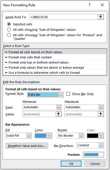
6 .4 . COLOUR SCALES
The Colour Scales option allows different shades of a colour to be used in a range of cells (see Figure 6.18). The greater or lesser intensity of the colour shows whether the data is higher or lower (see example in Table 6.9).
96
Basic Concepts in Pivot Tables
ISBN: 978-84-18432-98-9
DOI: http://dx.doi.org/10.6035/Sapientia179
Beatriz Forés Julián, Alba Puig Denia, Rafael Lapiedra Alcamí, Francisco Fermín Mallén Broch, José Mª Fernández YáñezFigure
It is also possible to use several colours with different intensities. For example, the highest values can be displayed by default in green and the lowest in yellow. Different intensities are also used inside the cells shown in green, so that the highest values appear in a darker green. The same applies to the cells in yellow (see Table 6.10).
Basic Concepts in Pivot Tables

97
Puig
ISBN: 978-84-18432-98-9 Beatriz Forés Julián, Alba
Denia, Rafael Lapiedra Alcamí, Francisco Fermín Mallén Broch, José Mª Fernández Yáñez DOI: http://dx.doi.org/10.6035/Sapientia179
Sum of Kilograms Quarter Product Quarter 1 Quarter 2 Grand Total Glass 12200 12150 24350 Metal 9100 8800 17900 Paper and cardboard 13350 12700 26050 Plastic 9400 8700 18100 Textile 5900 5750 11650 Grand Total 49950 48100 98050
6.18. Colour Scales menu Table 6.9. Example of a colour scale applying a single colour
Basic Concepts in Pivot Tables
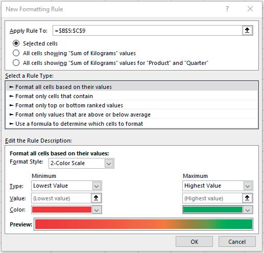
ISBN: 978-84-18432-98-9
Figure
98
Beatriz Forés Julián, Alba Puig Denia, Rafael Lapiedra Alcamí, Francisco Fermín Mallén Broch, José Mª Fernández Yáñez
of a colour scale applying two colours Sum of Kilograms Quarter Product Quarter 1 Quarter 2 Grand Total Glass 12200 12150 24350 Metal 9100 8800 17900 Paper and cardboard 13350 12700 26050 Plastic 9400 8700 18100 Textile 5900 5750 11650 Grand Total 49950 48100 98050
in other previous options, other rules can also be defined
DOI: http://dx.doi.org/10.6035/Sapientia179 Table 6.10. Example
As
(see Figure 6.19).
6.19. More formatting rules
6 .5 . ICON SETS
This option can be used to add an icon in each cell, which represents its value (see Figure 6.20).
Figure 6.20. Icon Sets
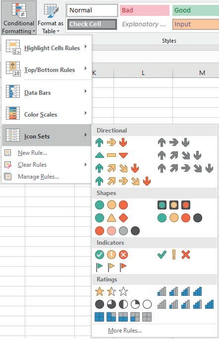
For example, coloured flags have been used in Table 6.10 below.
Table 6.10. Icon Sets example
99

Basic Concepts in Pivot Tables
ISBN: 978-84-18432-98-9
DOI: http://dx.doi.org/10.6035/Sapientia179
Beatriz Forés Julián, Alba Puig Denia, Rafael Lapiedra Alcamí, Francisco Fermín Mallén Broch, José Mª Fernández YáñezA green flag appears in the highest values, red in the lowest values and yellow in intermediate values.
It is also possible to apply the icons when illustrating the differences calculated between the real blood reserves and the anticipated values in the example of the blood bank mentioned above (see Annex II), thereby facilitating presentation of the results (see Table 6.11).

Table 6.11. Example difference between actual and forecast reserves
As in the previous sections, new custom rules can be defined to illustrate the icons (see Figure 6.21).
100
Basic Concepts in Pivot Tables
ISBN: 978-84-18432-98-9
DOI: http://dx.doi.org/10.6035/Sapientia179
Beatriz Forés Julián, Alba Puig Denia, Rafael Lapiedra Alcamí, Francisco Fermín Mallén Broch, José Mª Fernández YáñezFigure 6.21. Options in More Rules
However, there are some precautions that must be followed when using the conditional formatting option, as otherwise the results could be misinterpreted. For example, if a selection is not deleted before applying another section, the different formats will overlap and the result will not be the one desired.
6 .6 . NEW RULE
As discussed above, there are numerous options for applying conditional formatting to a set of cells. In addition to the predefined options that have been explained, it is possible to specify the design of custom conditional formats.

In this section, we will continue to use the example of waste collection, but now we will distinguish between the amounts collected for each type of product and month, as shown in the example in Table 6.12.
Basic Concepts in Pivot Tables
ISBN: 978-84-18432-98-9
DOI: http://dx.doi.org/10.6035/Sapientia179
101
Beatriz Forés Julián, Alba Puig Denia, Rafael Lapiedra Alcamí, Francisco Fermín Mallén Broch, José Mª Fernández Yáñez
Table 6.12. Starting pivot table example
Sum of Kilograms Month
Product
1 2 3 4 5 6 Grand Total
Glass 4200 4500 3500 6300 3700 2150 24350
Metal 3400 2600 3100 5100 2100 1600 17900
Paper and cardboard 4300 4550 4500 6450 3750 2500 26050
Plastic 3000 3200 3200 4500 2600 1600 18100
Textile 2100 1600 2200 3150 1500 1100 11650
Grand Total 17000 16450 16500 25500 13650 8950 98050
Next, we execute Conditional Formatting , New Rule and a dialog box like the one shown in Figure 6.22 appears.
Basic Concepts in Pivot Tables
ISBN: 978-84-18432-98-9
Figure 6.22 New formatting rule

102
Beatriz
DOI: http://dx.doi.org/10.6035/Sapientia179
Forés Julián, Alba Puig Denia, Rafael Lapiedra Alcamí, Francisco Fermín Mallén Broch, José Mª Fernández YáñezThis dialog box is divided into three blocks. In the first, the cell or cells in which the rule is to be applied must be specified. In the second, the rule type to be applied must be selected. Finally, the third block is used to define the format to be applied. Let us take a closer look at these options.
First, the new rule can be applied to the selected cells, those that show the total kilos, or as a last option, the cells that contain the sum of kilos for each Product and Month. This example uses the third possibility. Once this has been done, a rule type must be selected. We select Format all cells based on their values
Finally, the desired format for the cell will be specified. There are four options: 2-Color Scale , 3-Color Scale , Data Bars , or Icon Sets . In our example, we select the Icon Sets option as the format style, and then the 3 triangles option as the style.
For each icon (red triangle, yellow bar and green triangle), you can specify different cut points. Newer versions of Excel allow the icon style to be customized for each range of values.
In addition, selecting the icons using their Figures (instead of text) makes work easier than in previous versions of Excel.
Finally, once you have chosen the desired icon for each data range, you only need specify the values that you want to associate with each icon, e.g. green for values greater than 4,000 kg per month and red for values less than 2,000 kg per month (see Figure 6.23).
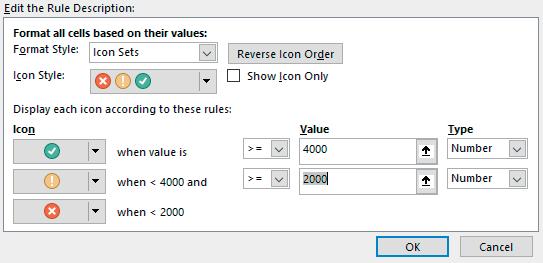
Figure 6.23. Format rule application example
The type of unit and the values that you want to appear in a specific format have therefore been selected. The result is presented in Table 6.13.
Basic Concepts in Pivot Tables
ISBN: 978-84-18432-98-9
DOI: http://dx.doi.org/10.6035/Sapientia179
103
Beatriz Forés Julián, Alba Puig Denia, Rafael Lapiedra Alcamí, Francisco Fermín Mallén Broch, José Mª Fernández Yáñez
Table 6.13. Result of applying the format rule
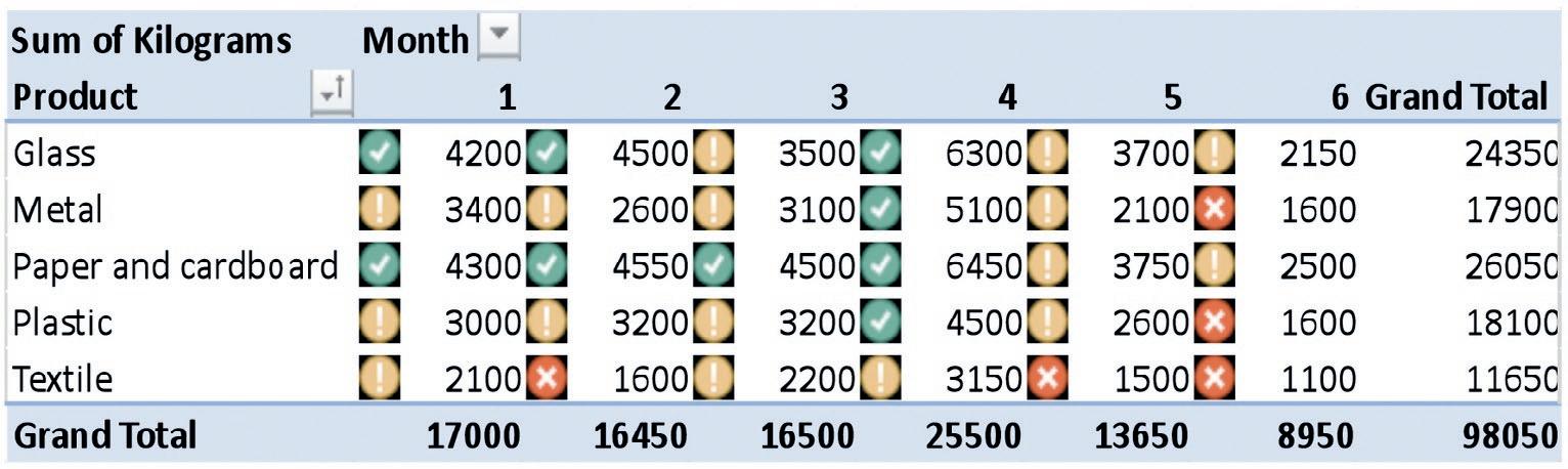
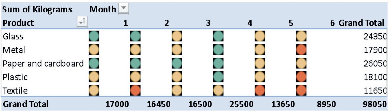
There is another interesting option, called Invert Icon Sort Order . You can use it reverse the order of the selected icons. Another interesting feature or option is Show Icon Only , which shows only the icons that do not have values in the table. The result of applying this option would be the following (Table 6.14).
Table 6.14. Example when applying the Show Icon Only option
As seen above, there are multiple possibilities and combinations for applying conditional formatting to the data in a table. After this brief introduction to the options, each user should explore other possibilities depending on their needs of.
6 .7 . CLEAR RULES
Sometimes it may be useful to remove the rules that have been created to apply conditional formats to pivot tables. This can be achieved with the Clear Rules option, which offers various options as shown in Figure 6.24 below.
Basic Concepts in Pivot Tables
ISBN: 978-84-18432-98-9
DOI: http://dx.doi.org/10.6035/Sapientia179
104
Beatriz Forés Julián, Alba Puig Denia, Rafael Lapiedra Alcamí, Francisco Fermín Mallén Broch, José Mª Fernández Yáñez
Figure 6.24. Options in Clear Rules
It is possible to choose between:
• Clearing the rules from a previously selected set or range of cells.
• Clearing the rules from the entire spreadsheet you are working on.
• Clearing rules from this table is applicable when using data in Excel table format, but not linked to a pivot table.
• Clearing rules from this pivot table is an option that allows you to delete the rules of the pivot table in which you have selected one or more cells.
6 .8 . CONDITIONAL FORMATTING RULES MANAGER
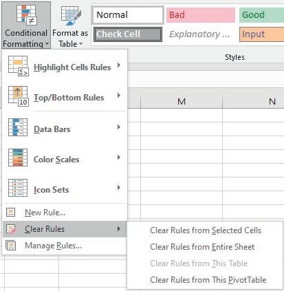
Conditional Formatting Rules Manager is used to change, create or delete rules created in a selected table or in others (see Figure 6.25).
Figure 6.25. Conditional Formatting Rules Manager

Basic Concepts in Pivot Tables
ISBN: 978-84-18432-98-9
DOI: http://dx.doi.org/10.6035/Sapientia179
105
Beatriz Forés Julián, Alba Puig Denia, Rafael Lapiedra Alcamí, Francisco Fermín Mallén Broch, José Mª Fernández Yáñez
Figures 6.26-6.27 below show the different options that will be obtained.
Figure 6.26. Create rules using New Formatting Rule


Basic Concepts in Pivot Tables
ISBN: 978-84-18432-98-9
Figure 6.27. Delete rules using Delete Rule
DOI: http://dx.doi.org/10.6035/Sapientia179
106
Beatriz Forés Julián, Alba Puig Denia, Rafael Lapiedra Alcamí, Francisco Fermín Mallén Broch, José Mª Fernández Yáñez
Chapter 7: Creating and designing charts with pivot tables: practical examples
As explained above, the layout and data that is displayed in a pivot table ca be changed. Pivot chart reports can also be created. Their main characteristic is their flexibility, since they also enable different designs and options to be used to present data.
For each pivot chart report, there is a pivot table report that uses the corresponding layout. The two reports share some fields, and when a change is made to the position of the fields in one of the reports, the same field in the other report is also modified.
7 .1 . ALTERNATIVES TO CREATING A PIVOT CHART
Continuing with the example of recycling product dumps, two different ways of creating a pivot chart are explained below (see Figure 7.1).
Basic Concepts in Pivot Tables
ISBN: 978-84-18432-98-9
DOI: http://dx.doi.org/10.6035/Sapientia179
107
Beatriz Forés Julián, Alba Puig Denia, Rafael Lapiedra Alcamí, Francisco Fermín Mallén Broch, José Mª Fernández Yáñez
7 .1 .1 .
Figure 7.1. Pivot chart creation options
Creating a Pivot Chart via the Insert, Pivot chart option
This option is used when the pivot table has not yet been created. It will be based on the data table shown below (see Annex II).
Table 7.1. Baseline data for creating a pivot chart
Year Quarter Month Province City Hospital
Planned reserve (number of blood donors planned)
Actual reserve (actual number of blood donors)
Difference (Actual reservePlanned reserve)
2018 Quarter 1 January Castellón Castellón Hospital General 165 182 17
2018 Quarter 1 January Castellón Castellón Hospital Provincial 180 200 20
2018 Quarter 1 January Castellón Castellón Centro 9 de Octubre 90 73 -17
2018 Quarter 1 January Castellón Vinaroz Hospital Comarcal de Vinaròs 110 140 30
2018 Quarter 1 January Castellón Vilareal Hospital La Plana 135 160 25
2018 Quarter 1 January Valencia Valencia Hospital Universitario La Fe 200 227 27
2018 Quarter 1 January Valencia Valencia Hospital Clínico Universitario 185 157 -28
2018 Quarter 1 January Valencia Valencia Hospital La Malvarrosa 105 149 44
2018 Quarter 1 January Valencia Sagunto Hospital Sagunto 140 144 4
2018 Quarter 1 January Valencia Onteniente Hospital General d'Ontinyent 115 109 -6
2018 Quarter 1 January Valencia Alcira Hospital La Ribera de Alzira 125 145 20
2018 Quarter 1 January Valencia Requena Hospital Requena 70 89 19
2018 Quarter 1 January Valencia Játiva Hospital Xàtiva "Lluís Alcanyís" 85 71 -14
2018 Quarter 1 January Alicante Alicante Hospital General de Alicante 145 155 10
2018 Quarter 1 January Alicante Alicante Hospital San Juan de Alicante 120 138 18
2018 Quarter 1 January Alicante Denia Hospital Dénia 165 167 2
To make the chart with Excel 2019, select Insert, Pivot Chart (see Figure 7.2). Now click again on the Pivot Chart option, and a dialog box will appear in which you have to specify the table or data range. If you had an active cell in the data table, this space would appear filled. If not, it would appear blank.

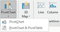
108
Basic Concepts in Pivot Tables
ISBN: 978-84-18432-98-9
Beatriz Forés Julián, Alba Puig Denia, Rafael Lapiedra Alcamí, Francisco Fermín Mallén Broch, José Mª Fernández Yáñez
DOI: http://dx.doi.org/10.6035/Sapientia179
Figure 7.2. Selecting and creating the pivot chart
After specifying the range of cells to be included in the chart, clicking OK will create the pivot chart. The result is shown in Figure 7.3. As above, the fact that the pivot table fields are related to those in the chart must be taken into account. The filters and selections in the graph are therefore those in the table, and vice versa.
Basic Concepts in Pivot Tables

ISBN: 978-84-18432-98-9
DOI: http://dx.doi.org/10.6035/Sapientia179
109
Beatriz Forés Julián, Alba Puig Denia, Rafael Lapiedra Alcamí, Francisco Fermín Mallén Broch, José Mª Fernández Yáñez
Figure 7.3. Creating a pivot chart
7 .1 .2 Creating a Pivot Chart using the Analyze, Pivot Chart option
This option is valid when a pivot table has already been defined. To generate the chart, first select one of the table cells (see Table 7.2).
Table 7.2. Example of the initial pivot table
Centro 9 de Octubre 540 503 -37
Hospital Clínico Universitario 1125 1046 -79 Hospital Comarcal de Vinaròs 635 635 0 Hospital Dénia 1055 1096 41 Hospital General 949 985 36 Hospital General de Alicante 905 962 57 Hospital General d'Ontinyent 680 645 -35 Hospital General Universitario de Elche 1195 1145 -50 Hospital La Malvarrosa 650 727 77 Hospital La Plana 780 758 -22 Hospital La Ribera de Alzira 695 712 17 Hospital Provincial 1090 1111 21 Hospital Requena 435 431 -4 Hospital Sagunto 845 879 34 Hospital San Juan de Alicante 715 689 -26 Hospital San Vicente del Raspeig 865 887 22 Hospital Torrevieja 955 955 0 Hospital Universitario La Fe 1195 1282 87 Hospital Vega Baja de Orihuela "Vega Baja" 780 741 -39 Hospital Xàtiva "Lluís Alcanyís" 525 548 23 Grand Total 16614 16737 123
Next select Analyze, Pivot Chart (select the created pivot table with the cursor), and you will see a dialog box like the one shown in Figure 7.4.
Basic Concepts in Pivot Tables
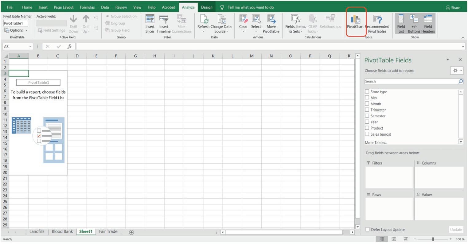
ISBN: 978-84-18432-98-9
DOI: http://dx.doi.org/10.6035/Sapientia179
110
Beatriz Forés Julián, Alba Puig Denia, Rafael Lapiedra Alcamí, Francisco Fermín Mallén Broch, José Mª Fernández Yáñez
Row Labels Sum of Planned reserve (number of blood donors planned) Sum of Actual reserve (actual number of blood donors) Sum of Difference (Actual reserve-Planned reserve)
Figure 7.4. Inserting a Pivot chart
There are different options (grouped column, three-dimensional columns, etc.) for each type of chart (column, line, circle, etc.). After selecting the desired combination, click on OK and the graph chosen will be displayed on the screen. Excel 2019 incorporates the filters of the different fields that are part of the graph (see Figure 7.5).

111
Basic Concepts in Pivot Tables
ISBN: 978-84-18432-98-9
DOI: http://dx.doi.org/10.6035/Sapientia179
Beatriz Forés Julián, Alba Puig Denia, Rafael Lapiedra Alcamí, Francisco Fermín Mallén Broch, José Mª Fernández YáñezFigure 7.5. Inserting a filter
The possibilities for editing a dynamic chart in Excel are the same as those of conventional charts in this application. Excel 2019 allows you to change the characteristics within the graph itself (incorporate titles, legend, trend lines, etc.). These options are accessed by means of the + sign (see Figure 7.6).


Basic Concepts in Pivot Tables
ISBN: 978-84-18432-98-9
Figure 7.6. Chart Elements options
DOI: http://dx.doi.org/10.6035/Sapientia179
112
Beatriz Forés Julián, Alba Puig Denia, Rafael Lapiedra Alcamí, Francisco Fermín Mallén Broch, José Mª Fernández Yáñez
If you select the sign with the brush for the style and colour options, Figure 7.7 below appears.
Figure 7.7. Style and Colour options
7 .2 . THE PIVOT CHART MENU
If you have followed the steps to create a chart from an existing pivot table, your screen will be similar to the one shown in Figure 7.8 below.

Figure 7.8. Pivot chart menu
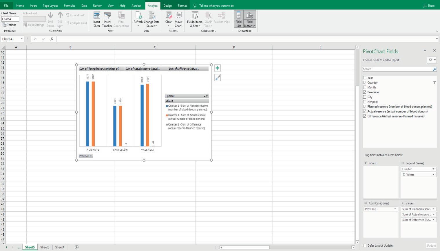
Basic Concepts in Pivot Tables
ISBN: 978-84-18432-98-9
DOI: http://dx.doi.org/10.6035/Sapientia179
113
Beatriz Forés Julián, Alba Puig Denia, Rafael Lapiedra Alcamí, Francisco Fermín Mallén Broch, José Mª Fernández Yáñez
The characteristics of each tab will be explained below.
7 .2 .1 . The Analyze tab
Figure 7.9 below shows the options that can be applied using the Analyze tab.
Figure 7.9. Analyze tab options
7 .2 .2 . The Design tab
Figure 7.10 shows the options that can be applied using the Design tab.
Figure 7.10. Chart designs
This tab gives the user flexibility to modify and adapt the features to their specific needs. As mentioned above, all these features are the same as those that can be applied to any chart that comes from an Excel data table.

Chart styles: allows the user to choose from a number of predefined chart types (see Figure 7.11).
Figure 7.11. Chart design styles
114

Basic Concepts in Pivot Tables
ISBN: 978-84-18432-98-9
DOI: http://dx.doi.org/10.6035/Sapientia179
Beatriz Forés Julián, Alba Puig Denia, Rafael Lapiedra Alcamí, Francisco Fermín Mallén Broch, José Mª Fernández YáñezData : to change the order of the data or to select others (see Figure 7.12).
Figure 7.12. Data selection
Change chart type: if a chart is selected, this option allows you to modify its type (see Figure 7.13).


Figure 7.13. Change Chart Type

Move location : used to change the selected graph to another tab in the same book (see Figure 7.14).
Basic Concepts in Pivot Tables
ISBN: 978-84-18432-98-9
Figure 7.14. Move Chart
DOI: http://dx.doi.org/10.6035/Sapientia179
115
Beatriz Forés Julián, Alba Puig Denia, Rafael Lapiedra Alcamí, Francisco Fermín Mallén Broch, José Mª Fernández Yáñez
7 .2 .3 . The Format tab
The Format tab also contains different options which will be explained below.

Active selection : used to apply or reset part formats of the selected graph (see Figure 7.15).
Figure 7.15. Active selection
Insert shapes (see Figure 7.16).
Figure 7.16. Insert Shapes
Shape and Wordart styles (see Figure 7.17).

Figure 7.17. Shape Styles
Organize is used to change the position graph according to the option chosen (see Figure 7.18).
Basic Concepts in Pivot Tables
ISBN: 978-84-18432-98-9
DOI: http://dx.doi.org/10.6035/Sapientia179
116
Beatriz Forés Julián, Alba Puig Denia, Rafael Lapiedra Alcamí, Francisco Fermín Mallén Broch, José Mª Fernández Yáñez
Figure 7.18. Chart organization
Size is used to modify the width and/or height of the chart (see Figure 7.19).
Figure 7.19. Changing the size of the chart
7 .3 . CHART EXAMPLES
To explain this section, we will use the example of the blood bank in the hospitals in the Valencian Community. Based on this example, let us assume that we have the data shown in Table 7.3 below.
Table 7.3. Initial data
Basic Concepts in Pivot Tables
ISBN: 978-84-18432-98-9
DOI: http://dx.doi.org/10.6035/Sapientia179
117
Beatriz Forés Julián, Alba Puig Denia, Rafael Lapiedra Alcamí, Francisco Fermín Mallén Broch, José Mª Fernández Yáñez
Year Month Province Planned reserve (number of blood donors planned) Actual reserve (actual number of blood donors) 2018 1 Alicante 1,055 1,066 2018 1 Castellón 680 755 2018 1 Valencia 1,025 1,091 2018 2 Alicante 1,030 1,003
Year Month Province
Planned reserve (number of blood donors planned)
Actual reserve (actual number of blood donors)
2018 2 Castellón 639 598 2018 2 Valencia 965 968 2018 3 Alicante 1,090 939 2018 3 Castellón 665 635 2018 3 Valencia 1,030 1,005 2018 4 Alicante 1,100 1,063 2018 4 Castellón 665 662 2018 4 Valencia 1,035 1,035 2018 5 Alicante 1,080 1,277 2018 5 Castellón 680 669 2018 5 Valencia 1,035 1,091 2018 6 Alicante 1,115 1,139 2018 6 Castellón 665 673 2018 6 Valencia 1,060 1,080
The data are described below:
Year Year in which donations take place Month Month in which donations are made Province Province of the hospital where donations are made Planned reserve Number of donors expected in each province Actual reserve Number of actual donors in each province
This table allows you to compare the number of actual donations by year, month and province, as well as the number of expected donors versus actual donors. Our goal is to analyze this data by creating a graph from a pivot table.
Basic Concepts in Pivot Tables
ISBN: 978-84-18432-98-9
Beatriz Forés Julián, Alba Puig Denia, Rafael Lapiedra Alcamí, Francisco Fermín Mallén Broch, José Mª Fernández Yáñez
DOI: http://dx.doi.org/10.6035/Sapientia179
118
• Generating a graph from a pivot table
A very simple pivot table will be used, based on the previous example. The pivot table will be created to simply display the quarter, along with the total number of donors (see Table 7.4).

Table 7.4. Initial pivot table example
Row Labels Sum of Actual reserve (actual number of blood donors)
Quarter 1 8219
Quarter 2 8518
Grand Total 16737
With an active cell of the previous pivot table, you must select the option Pivot chart and choose one of the chart types. For example, we select the Stacked Column Chart and obtain what is shown in Figure 7.20.
Figure 7.20. Pivot stacked column chart
Figures 7.21-7.27 show different types of analysis that can be applied on the basis of our pivot table.
Basic Concepts in Pivot Tables
ISBN: 978-84-18432-98-9
DOI: http://dx.doi.org/10.6035/Sapientia179
119
Beatriz Forés Julián, Alba Puig Denia, Rafael Lapiedra Alcamí, Francisco Fermín Mallén Broch, José Mª Fernández Yáñez
Figure 7.21. Analysis of the actual number of donors
Figure 7.22. Analysis of the differences between the number of donors per month in Valencia
Figure 7.23. Number of donors per month
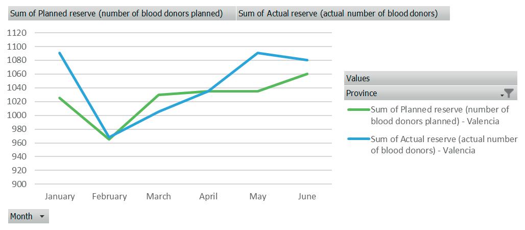


120
Basic Concepts in Pivot Tables
ISBN: 978-84-18432-98-9
DOI: http://dx.doi.org/10.6035/Sapientia179
Beatriz Forés Julián, Alba Puig Denia, Rafael Lapiedra Alcamí, Francisco Fermín Mallén Broch, José Mª Fernández YáñezFigure 7.24. Number of donors per month with a linear trend over the year
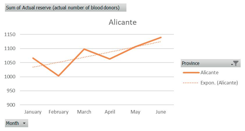

Figure 7.25. Number of donors per month with an exponential trend over the year
121
Basic Concepts in Pivot Tables
ISBN: 978-84-18432-98-9
DOI: http://dx.doi.org/10.6035/Sapientia179
Beatriz Forés Julián, Alba Puig Denia, Rafael Lapiedra Alcamí, Francisco Fermín Mallén Broch, José Mª Fernández YáñezFigure 7.26. Difference between the actual and expected number of donors

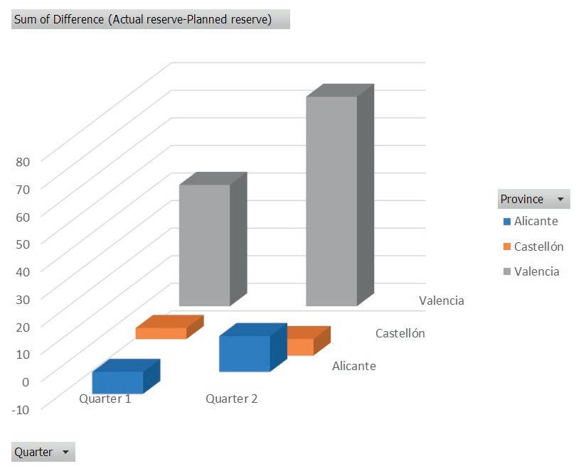
Figure 7.27. Difference between the actual and planned number of donors (II)
Basic Concepts in Pivot Tables
ISBN: 978-84-18432-98-9
DOI: http://dx.doi.org/10.6035/Sapientia179
122
Beatriz Forés Julián, Alba Puig Denia, Rafael Lapiedra Alcamí, Francisco Fermín Mallén Broch, José Mª Fernández Yáñez
Chapter 8: A practical example of the application of pivot tables
We start with the example of a company that sells fair-trade products. In order to be designated fair-trade products, the goods must comply with a series of requirements, including offering decent working conditions, rejecting child exploitation, promoting gender equality and care for the environment.
An increasing number of products meet these requirements, but in this example we will focus on one specific case. Let us suppose that our organization distributes five different products related to the food sector (chocolate, coffee, fruit juice, wine and oil).
The organization has 5 physical stores in some of Spain’s largest cities: Barcelona, Bilbao, Madrid, Seville and Valencia. It also has itinerant stores, as it attends various gastronomic fairs every month in cities all over Spain, and has attended events in Badajoz, Cádiz, Castellón, Córdoba, Gijón, Huelva, Logroño, Málaga, O Cebreiro, Potes, Santillana del Mar and Teruel every year since 2013.
Our organization has collected data on the sales of each product in each city since 2013 (Table 8.1.). In addition to the city, the table shows the type of store (physical or itinerant), the month (both numerically and qualitatively), the quarter, semester, year, type of product and monthly sales in Euros.
Basic Concepts in Pivot Tables
ISBN: 978-84-18432-98-9
DOI: http://dx.doi.org/10.6035/Sapientia179
123
Beatriz Forés Julián, Alba Puig Denia, Rafael Lapiedra Alcamí, Francisco Fermín Mallén Broch, José Mª Fernández Yáñez
Table 8.1. Sales (in Euros) of fair-trade products in different Spanish cities
The result is a spreadsheet that contains more than 2000 rows, so pivot tables can be used to analyze and better understand various aspects of the organization’s work.
However, this raises a series of questions:
1. What were the trends in total sales between 2013 and 2018, and in the sales of each type of product?
2. How does the distribution of the sales at trade fairs compare to sales at permanent distribution points? What is the relative weight of the sales in each of these types of stores?
3. How have total sales changed in each city?
4. What is the star product in each city, and what is its relative weight within the total sales of each city?
5. Taking all the data series into account, in which months were there the most sales of each type of product? Is the same pattern present in fixed and itinerant stores?
6. Considering only the data for 2018, which locations were the best/worst for each type of product marketed?
7. In the 2018 data, which three cities had the highest and lowest sales? Can we obtain a ranking of cities classified according to their 2018 sales?
All these questions and many more can be answered by taking advantage of the knowledge obtained from reading this book. Let us look one by one at some
Basic Concepts in Pivot Tables

ISBN: 978-84-18432-98-9
DOI: http://dx.doi.org/10.6035/Sapientia179
124
Beatriz Forés Julián, Alba Puig Denia, Rafael Lapiedra Alcamí, Francisco Fermín Mallén Broch, José Mª Fernández Yáñez
of the ways to exploit and present the data in a way that satisfies the information needs of our company.
Question 1. What were the trends in total sales between 2013 and 2018, and in the sales of each type of product?
Using the conditional format (data bars) on the pivot table, we can obtain the summary presented in Table 8.2 as a result. In addition to the quantities, it contains a bar that shows the continued growth of sales in the years analyzed. For greater clarity, a dynamic graph can also be produced using this information if desired (Figure 8.1.).
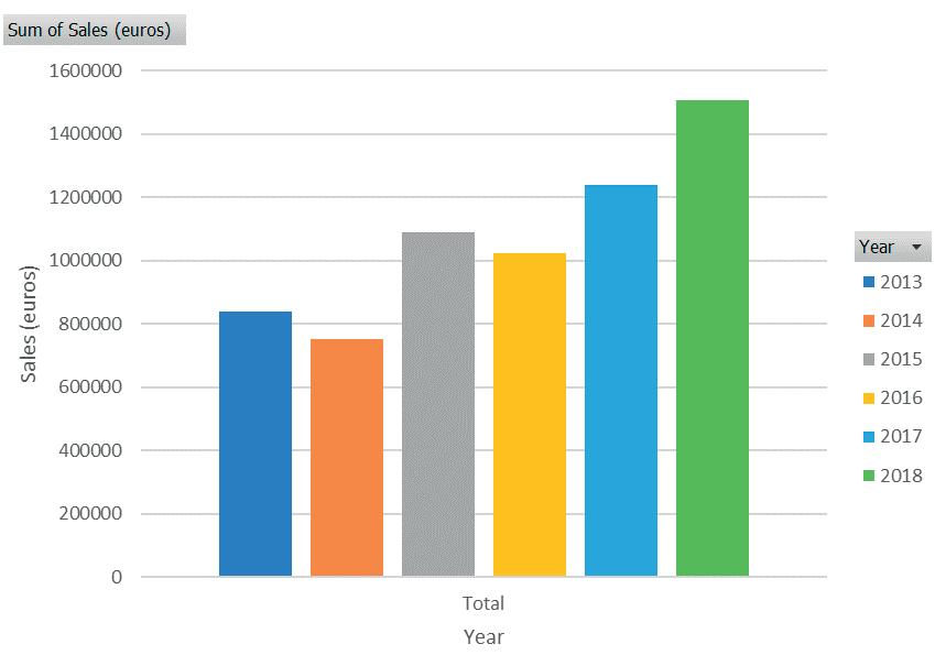
Table 8.2. Total sales (2013-2018)
Basic Concepts in Pivot Tables
ISBN: 978-84-18432-98-9
Figure 8.1. Annual sales (2013-2018)
DOI: http://dx.doi.org/10.6035/Sapientia179
125
Beatriz Forés Julián, Alba Puig Denia, Rafael Lapiedra Alcamí, Francisco Fermín Mallén Broch, José Mª Fernández Yáñez
Column Labels 2013 2014 2015 2016 2017 2018 Grand Total
of Sales (euros) 840614.41 751679.51 1088369.30 1025139.52 1239424.57 1508892.57 6454119.88
Sum
By slightly modifying the pivot table, we can access the details of annual sales for each product marketed (Table 8.3.). The data are displayed in Figure 8.2.
Table 8.3. Annual sales by product type
Sum of Sales (euros) Column Labels
Row Labels 2013 2014 2015 2016 2017 2018 Grand Total
Chocolate 57330.10 66419.01 68855.08 69914.75 81101.08 94077.19 437697.21
Coffee 110361.72 123820.46 145261.89 134587.46 168234.41 210293.07 892559.01
Fruit juice 106019.34 109898.10 147574.42 129291.88 152564.44 180025.98 825374.16
Olive oil 200816.23 183673.38 219561.12 244897.84 257142.72 269999.90 1376091.19
Wine 366087.02 267868.55 507116.80 446447.59 580381.92 754496.43 2922398.32
Grand Total 840614.41 751679.51 1088369.30 1025139.52 1239424.57 1508892.57 6454119.88
Figure 8.2. Annual sales by product type

Question 2. How does the distribution of the sales at trade fairs compare to sales at permanent distribution points? What is the relative weight of the sales in each of these types of stores?
Table 8.4 summarizes the information in absolute values, while Table 8.5 does so in relative values. As can be seen, sales at both permanent and itinerant distribution points increased over the years studied. On the other hand, the
126
Basic Concepts in Pivot Tables
ISBN: 978-84-18432-98-9
Beatriz
DOI: http://dx.doi.org/10.6035/Sapientia179
Forés Julián, Alba Puig Denia, Rafael Lapiedra Alcamí, Francisco Fermín Mallén Broch, José Mª Fernández Yáñezproportion between both types of store remains more or less constant, as the itinerant roaming stores only account for approximately 6% of the total sales in each year. Figure 8.3 shows the distribution of sales between the two types of store for 2018.

Table 8.4. Sales: itinerant vs. permanent (absolute values)
Sum of Sales (euros) Column Labels
Row Labels 2013 2014 2015 2016 2017 2018 Grand Total
Itinerant 51716.22 49611.12 68279.77 63068.56 75870.17 91698.01 400243.85 Permanent 788898.19 702068.38 1020089.54 962070.96 1163554.40 1417194.56 6053876.03
Grand Total 840614.41 751679.51 1088369.30 1025139.52 1239424.57 1508892.57 6454119.88
Table 8.5. Sales: itinerant vs. permanent (relative values)
Sum of Sales (euros) Column Labels
Row Labels 2013 2014 2015 2016 2017 2018 Grand Total
Itinerant
6.15% 6.60% 6.27% 6.15% 6.12% 6.08% 6.20% Permanent 93.85% 93.40% 93.73% 93.85% 93.88% 93.92% 93.80% Grand Total 100.00% 100.00% 100.00% 100.00% 100.00% 100.00% 100.00%
Figure 8.3. Relative weight of sales in permanent vs. itinerant stores (2018)
127
Basic Concepts in Pivot Tables
ISBN: 978-84-18432-98-9
DOI: http://dx.doi.org/10.6035/Sapientia179
Beatriz Forés Julián, Alba Puig Denia, Rafael Lapiedra Alcamí, Francisco Fermín Mallén Broch, José Mª Fernández YáñezQuestion 3. How have total sales changed in each city?
To facilitate interpretation of the results, a distinction has again been made between fixed (Table 8.6.) and itinerant distribution centres (Table 8.7.), showing the detail of sales for each city and year available in each case. It has also been represented graphically (Figures 8.4. and 8.5.)

Table 8.6. Sales by city (permanent stores)
Store type Permanent
Sum of Sales (euros) Column Labels
Row Labels 2013 2014 2015 2016 2017 2018 Grand Total
Barcelona 212924.59 182741.60 241969.47 259664.13 316737.24 389108.77 1603145.79 Bilbao 122801.43 113981.65 177893.94 149757.84 179495.28 216585.15 960515.29 Madrid 220304.59 190067.60 316285.04 268664.13 327429.24 401876.18 1724626.77 Sevilla 125043.79 116185.77 156773.47 152492.43 182420.32 219707.55 952623.34 Valencia 107823.79 99091.77 127167.62 131492.43 157472.32 189916.91 812964.84
Grand Total 788898.19 702068.38 1020089.54 962070.96 1163554.40 1417194.56 6053876.03
Figure 8.4. Sales by city (permanent stores)
128
Basic Concepts in Pivot Tables
ISBN: 978-84-18432-98-9
DOI: http://dx.doi.org/10.6035/Sapientia179
Beatriz Forés Julián, Alba Puig Denia, Rafael Lapiedra Alcamí, Francisco Fermín Mallén Broch, José Mª Fernández YáñezTable 8.7. Sales by city (itinerant stores)
Store type Itinerant
Sum of Sales (euros) Column Labels
Row Labels 2013 2014 2015 2016 2017 2018 Grand Total
Badajoz
3821.89 3687.86 6325.42 4660.84 5614.02 6790.10 30900.13 Cádiz 3485.00 3370.37 4639.16 4250.00 5113.65 6178.84 27037.02
Castellón 4443.39 4297.23 6056.25 5418.77 6519.91 7878.01 34613.57
Córdoba 4094.89 3951.28 5147.83 4993.77 6015.01 7275.12 31477.91 Gijón 8189.75 7902.54 4744.08 9987.50 12030.02 14550.22 57404.11
Huelva 5459.84 5268.36 9488.13 6658.34 8020.00 9700.14 44594.81
Logroño 5350.63 5162.98 4427.80 6525.16 7859.60 9506.14 38832.31
Málaga 5227.50 5055.55 4037.50 6375.00 7670.48 9268.25 37634.28
O Cebreiro 2002.17 1878.69 2889.59 2441.67 2908.86 3489.05 15610.02
Potes 3142.66 2911.81 14563.54 3832.51 4679.22 5743.80 34873.54
Santillana del Mar 2494.17 2367.09 3640.88 3041.67 3621.66 4340.22 19505.69
Teruel 4004.33 3757.36 2319.59 4883.33 5817.74 6978.12 27760.47
Grand Total 51716.22 49611.12 68279.77 63068.56 75870.17 91698.01 400243.85
Figure 8.5. Sales by city (itinerant stores)
Question 4. What is the star product in each city, and what is its relative weight within the total sales of each city?
Although the form of the question means it is necessary to perform an analysis for each city, we initially analyzed the case of the Barcelona store (Table 8.8.). When showing the data for the other cities, it would be sufficient to modify the filter that appears at the top of the pivot table, indicating the city for which the
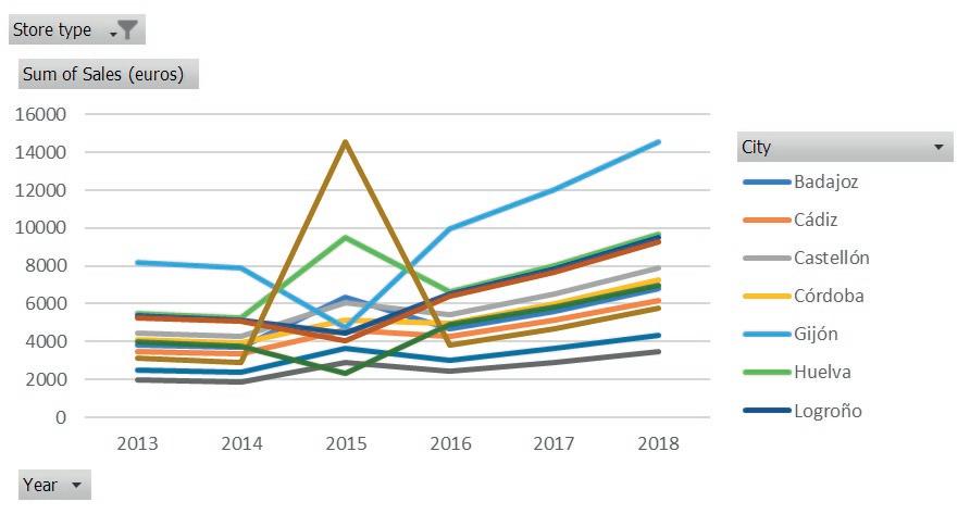
129
Basic Concepts in Pivot Tables
ISBN: 978-84-18432-98-9
Beatriz
DOI: http://dx.doi.org/10.6035/Sapientia179
Forés Julián, Alba Puig Denia, Rafael Lapiedra Alcamí, Francisco Fermín Mallén Broch, José Mª Fernández Yáñezinformation is desired. Figure 8.6 shows the evolution sales for each type of product in this store. The sales trend is upwards for all the products marketed between 2013 and 2018, and the star product every year is clearly wine.

Table 8.8. Sales by product in the Barcelona store (2013-2018)
City Barcelona Store type Permanent
Sum of Sales (euros) Column Labels
Row Labels
2013 2014 2015 2016 2017 2018 Grand Total
Chocolate 8188.90 9487.14 9366.28 9986.46 11584.29 13437.77 62050.83
Coffee 21541.86 24168.92 22895.29 26270.56 32838.22 41047.79 168762.63
Fruit juice 19221.96 19925.20 22436.03 23441.41 27660.87 32639.82 145325.29
Olive oil 50189.07 45904.64 57829.85 61206.18 64266.48 67479.81 346876.02
Wine 113782.81 83255.71 129442.02 138759.52 180387.38 234503.58 880131.01
Grand Total 212924.59 182741.60 241969.47 259664.13 316737.24 389108.77 1603145.79
Figure 8.6. Sales by product in the Barcelona store (2013-2018)
Following the example of the Barcelona store, another possibility is to obtain data exclusively for the last year available (Table 8.9) and from there, to produce a graph that better represents how the sales of each type of product are distributed (Figure 8.7.). In Table 8.9., the conditional format option has also used icons to highlight the highest data.
130
Basic Concepts in Pivot Tables
ISBN: 978-84-18432-98-9
DOI: http://dx.doi.org/10.6035/Sapientia179
Beatriz Forés Julián, Alba Puig Denia, Rafael Lapiedra Alcamí, Francisco Fermín Mallén Broch, José Mª Fernández YáñezTable 8.9. Product sales in Barcelona store (2018)
Figure 8.7. Sales by product in Barcelona (2013-2018)
Question 5. Taking all the data series into account, in which months were there the most sales of each type of product? Is the same pattern present in fixed and itinerant stores?
First, Table 8.10 presents the sales of each product type by month. The conditional format has been used to highlight the best and worst data for each

131

Basic Concepts in Pivot Tables
ISBN: 978-84-18432-98-9
DOI: http://dx.doi.org/10.6035/Sapientia179
Beatriz Forés Julián, Alba Puig Denia, Rafael Lapiedra Alcamí, Francisco Fermín Mallén Broch, José Mª Fernández Yáñeztype of product. For example, for olive oil, the best month is June (highlighted in green), while the worst is September (highlighted in red). Reading the information presented in Tables 8.11 and 8.12 tells us that the pattern of best and worst months is not the same in itinerant and permanent stores. As can be seen, March is the worst month for all products except for olive oil in itinerant stores. Nor is there a similar pattern for the best month for each type of product when distinguishing between one type of shop and another.
Table 8.10. Sales of each type of product (best and worst month without distinguishing between the type of store) Sum
Chocolate 33637.63 35028.41 39712.82 45408.31 43077.04 41648.23 34505.40 28449.69 27468.09 29281.79 32311.91 47167.91 437697.21
Coffee 59766.47 55504.18 59167.91 65527.64 73293.73 86054.63 75085.71 65430.09 58544.93 72370.53 92229.61 129583.58 892559.01 Fruit
39938.91 39708.04 41733.54 47706.58 56667.36 67145.09 79335.26 93213.14 124975.20 97760.88 74278.09 62912.07 825374.16 Olive
111368.24 126816.51 143309.44 154547.53 159161.29 171106.48 125033.93 92738.89 65924.01 68333.62 73221.38 84529.88 1376091.19
Wine 236071.97 197822.77 183268.00 199362.95 212199.31 239977.25 262507.43 284493.08 322133.57 249871.01 191534.73 343156.26 2922398.32 Grand Total 480783.22 454879.90 467191.71 512553.01 544398.72 605931.66 576467.72 564324.88 599045.81 517617.84 463575.72 667349.69 6454119.88 Table 8.11.
Chocolate 30091.54 32327.15 37596.25 41708.76 39115.86 36019.97 29329.25 23857.68 19134.03 22807.89 27826.06 41530.25 381344.69 Coffee 51495.87 51887.82 56582.96 60946.74 69601.14 81090.49 70535.82 61466.51 51346.58 66815.27 88378.74 124721.84 834869.77 Fruit
36377.94 36974.84 39576.05 43933.10 48692.25 54791.36 67969.04 82592.13 105511.73 82629.22 63793.72 49743.17 712584.56
Olive oil 106020.81 122599.84 139527.21 147825.43 155524.14 167009.27 121236.38 89451.76 60048.23 63700.44 70013.94 80540.69 1323498.14
Wine 221923.53 191584.56 178299.22 190378.50 204428.30 229386.30 252783.67 275478.90 305601.13 237070.20 182663.13 331981.42 2801578.87
Grand Total 445909.68 435374.21 451581.69 484792.54 517361.70 568297.38 541854.16 532846.98 541641.70 473023.03 432675.59 628517.37 6053876.03
Chocolate 3546.09 2701.26 2116.57 3699.55 3961.17 5628.26 5176.15 4592.00 8334.06 6473.90 4485.85 5637.66 56352.52
8270.60 3616.35 2584.95 4580.90 3692.59 4964.14 4549.89 3963.58 7198.35 5555.26 3850.88 4861.74 57689.24
3560.97 2733.20 2157.49 3773.48 7975.11 12353.73 11366.21 10621.01 19463.47 15131.66 10484.37 13168.89 112789.60 Olive oil 5347.44 4216.67 3782.23 6722.09 3637.14 4097.21 3797.55 3287.13 5875.78 4633.18 3207.43 3989.19 52593.04 Wine 14148.44 6238.21 4968.78 8984.44 7771.01 10590.94 9723.76 9014.18 16532.44 12800.81 8871.60 11174.83 120819.45 Grand Total 34873.54 19505.69 15610.02 27760.47 27037.02 37634.28 34613.57 31477.91 57404.11 44594.81 30900.13 38832.31 400243.85
Question 6. Considering only the data for 2018, which locations were the best/ worst for each type of product marketed?
In our original table (see Table 8.1.) there is a column in which the location number is specified. If this column had not been there, one possibility would have been to use the “Group selection” option presented in section 2.4. Another
132
Basic Concepts in Pivot Tables
ISBN: 978-84-18432-98-9
Beatriz
DOI: http://dx.doi.org/10.6035/Sapientia179
Forés Julián, Alba Puig Denia, Rafael Lapiedra Alcamí, Francisco Fermín Mallén Broch, José Mª Fernández Yáñezof Sales (euros) Column Labels
Labels January February March April May June July August September October November December Grand Total
Row
juice
oil
Sales of each type of product
worst month, permanent stores) Store type Permanent Sum of Sales (euros) Column Labels Row Labels January February March April May June July August September October November December Grand Total
juice
(best and
Itinerant
of Sales (euros) Column Labels Row Labels January February March April May June July August September October November December Grand Total
Fruit juice
Table 8.12. Sales of each type of product (best and worst month, itinerant stores) Store type
Sum
Coffee
is to create it using the conditional function IF from the column where the month number is specified.
Leaving these considerations aside, we have used colour scales to highlight the information being sought. The information has again been divided into three tables. The first does not distinguish between the types of stores (Table 8.13.) while the others do (Tables 8.14. and 8.15.)
As the conditional format has been used in this example, the colour scale must be interpreted, row by row, i.e. product by product. In addition, the colours chosen should be interpreted in terms of a traffic light: the data in green are the most positive (the more positive, the greater the intensity of the green colour) and the data in red are negative (the more negative, the greater the intensity of the red). The data shown in yellow are average data within the series.
If we look at the data summarized in Table 8.13 and at the line where the oil sales data by location appears, we can see that two data in green are highlighted, and the colour of the second location is more intense, which indicates that this is the best data. The worst location, which is the fourth, is shaded in red. The other lines should be interpreted in a similar way.
Table 8.13. Quarterly sales by product type (2018)
Store type (All) Year 2018 Sum
Chocolate 23260.61 27881.94 19198.87 23735.77 94077.19 Coffee 39911.93 53481.37 46152.76 70747.01 210293.07 Fruit juice 26261.16 38078.98 66141.74 49544.10 180025.98 Olive oil 75108.26 96140.61 53832.31 44918.72 269999.90 Wine 155064.93 170135.84 227012.25 202283.41 754496.43 Grand Total 319606.89 385718.74 412337.93 391229.01 1508892.57
133
Basic Concepts in Pivot Tables
ISBN: 978-84-18432-98-9
DOI: http://dx.doi.org/10.6035/Sapientia179
Beatriz Forés Julián, Alba Puig Denia, Rafael Lapiedra Alcamí, Francisco Fermín Mallén Broch, José Mª Fernández Yáñezof Sales
Column
Labels Trimester 1 Trimester 2 Trimester 3 Trimester 4 Grand
(euros)
Labels Row
Total
Table 8.14. Quarterly sales by product type: permanent stores (2018)
Store type Permanent Year 2018
Sum of Sales (euros) Column Labels
Row Labels Trimester 1 Trimester 2 Trimester 3 Trimester 4 Grand Total
Chocolate 21707.71 24880.13 15184.27 20251.58 82023.69 Coffee 37155.18 50204.02 42287.91 67413.06 197060.17 Fruit juice 24626.75 32280.80 56543.23 41075.16 154525.94 Olive oil 72858.30 93309.02 51245.84 42691.86 260105.02 Wine 149685.88 162619.56 217373.33 193800.97 723479.74
Grand Total 306033.82 363293.53 382634.58 365232.63 1417194.56
Table 8.15. Quarterly sales by product type: itinerant stores (2018)
Store type Itinerant Year 2018
Sum of Sales (euros) Column Labels
Row Labels Trimester 1 Trimester 2 Trimester 3 Trimester 4 Grand Total
Chocolate 1552.90 3001.81 4014.60 3484.19 12053.50 Coffee 2756.75 3277.35 3864.85 3333.95 13232.90 Fruit juice 1634.41 5798.18 9598.51 8468.94 25500.04 Olive oil 2249.96 2831.59 2586.47 2226.86 9894.88 Wine 5379.05 7516.28 9638.92 8482.44 31016.69
Grand Total 13573.07 22425.21 29703.35 25996.38 91698.01
Question 7. In the 2018 data, which three cities had the highest and lowest sales? Can we obtain a ranking of cities classified according to their 2018 sales?
On this occasion, we apply the conditional format to the column showing the grand total (see Table 8.16.), indicating that it highlights the three best and the three worst data using green and red respectively. In other words, in this example two rules have been created - one for the most positive data and another for the most negative, with a different format specified in each case. If the three data had not been highlighted in each case, it would also have been useful to apply the colour scale option in the column with the grand total (see Table 8.17.).
134
Basic Concepts in Pivot Tables
ISBN: 978-84-18432-98-9
Beatriz Forés Julián, Alba Puig Denia, Rafael Lapiedra Alcamí, Francisco Fermín Mallén Broch, José Mª Fernández Yáñez
DOI: http://dx.doi.org/10.6035/Sapientia179
Table 8.16. Three cities with the highest and lowest sales (2018)
Sum of Sales (euros) Column Labels
Row Labels Trimester 1 Trimester 2 Trimester 3 Trimester 4 Grand Total
Badajoz 6790.10 6790.10 Barcelona 83332.29 98499.15 107121.93 100155.40 389108.77 Bilbao 46565.46 56413.82 57250.72 56355.15 216585.15 Cádiz 6178.84 6178.84 Castellón 7878.01 7878.01 Córdoba 7275.12 7275.12 Gijón 14550.22 14550.22 Huelva 9700.14 9700.14 Logroño 9506.14 9506.14 Madrid 86524.12 101691.02 110313.78 103347.26 401876.18 Málaga 9268.25 9268.25
O Cebreiro 3489.05 3489.05 Potes 5743.80 5743.80
Santillana del Mar 4340.22 4340.22 Sevilla 48529.81 57068.60 57697.90 56411.24 219707.55 Teruel 6978.12 6978.12 Valencia 41082.14 49620.94 50250.25 48963.58 189916.91
Grand Total 319606.89 385718.74 412337.93 391229.01 1508892.57
Table 8.17. Cities with the highest and lowest sales (2018)
Sum of Sales (euros) Column Labels
Row Labels Trimester 1 Trimester 2 Trimester 3 Trimester 4 Grand Total
Badajoz 6790.10 6790.10 Barcelona 83332.29 98499.15 107121.93 100155.40 389108.77 Bilbao 46565.46 56413.82 57250.72 56355.15 216585.15 Cádiz 6178.84 6178.84 Castellón 7878.01 7878.01 Córdoba 7275.12 7275.12 Gijón 14550.22 14550.22 Huelva 9700.14 9700.14 Logroño 9506.14 9506.14 Madrid 86524.12 101691.02 110313.78 103347.26 401876.18 Málaga 9268.25 9268.25
O Cebreiro 3489.05 3489.05 Potes 5743.80 5743.80
Santillana del Mar 4340.22 4340.22 Sevilla 48529.81 57068.60 57697.90 56411.24 219707.55
Teruel 6978.12 6978.12 Valencia 41082.14 49620.94 50250.25 48963.58 189916.91
Grand Total 319606.89 385718.74 412337.93 391229.01 1508892.57
135
Basic Concepts in Pivot Tables
ISBN: 978-84-18432-98-9
DOI: http://dx.doi.org/10.6035/Sapientia179
Beatriz Forés Julián, Alba Puig Denia, Rafael Lapiedra Alcamí, Francisco Fermín Mallén Broch, José Mª Fernández YáñezAnother way to answer this question would be to obtain the percentage of sales compared to the 2018 total for each city. By doing so, we would see that Barcelona and Madrid are the cities where most sales were made in 2018 (around 25% in each case), followed by Seville (around 15% of total sales in 2018). At the bottom, O Cebreiro, Potes and Santillana del Mar have sales that do not account for 1% of the total sales in 2018.
Table 8.18. Percentage of sales compared to the total for each city (2018)
Row Labels Sum of Sales
(euros)
Badajoz 0.45%
Barcelona 25.79% Bilbao 14.35% Cádiz 0.41% Castellón 0.52% Córdoba 0.48% Gijón 0.96% Huelva 0.64% Logroño 0.63% Madrid 26.63% Málaga 0.61% O Cebreiro 0.23% Potes 0.38% Santillana del Mar 0.29% Sevilla 14.56% Teruel 0.46% Valencia 12.59% Grand Total 100.00%
We can make a ranking in two ways, either by ordering the data from highest to lowest (Table 8.19.), or by adding a column showing the classified values (Table 8.20.).
Basic Concepts in Pivot Tables
ISBN: 978-84-18432-98-9
DOI: http://dx.doi.org/10.6035/Sapientia179
136
Beatriz Forés Julián, Alba Puig Denia, Rafael Lapiedra Alcamí, Francisco Fermín Mallén Broch, José Mª Fernández Yáñez
Basic Concepts in Pivot Tables
ISBN: 978-84-18432-98-9
Table 8.19. Percentage of sales made in each city (2018)
Year 2018
Row Labels Sum of Sales (euros) Madrid 26.63%
Barcelona 25.79% Sevilla 14.56% Bilbao 14.35% Valencia 12.59% Gijón 0.96% Huelva 0.64% Logroño 0.63% Málaga 0.61% Castellón 0.52% Córdoba 0.48% Teruel 0.46% Badajoz 0.45% Cádiz 0.41% Potes 0.38% Santillana del Mar 0.29% O Cebreiro 0.23%
Grand Total 100.00%
Table 8.20. Percentage and ranking of sales made in each city (2018)
137
Beatriz
DOI: http://dx.doi.org/10.6035/Sapientia179
Forés Julián, Alba Puig Denia, Rafael Lapiedra Alcamí, Francisco Fermín Mallén Broch, José Mª Fernández YáñezBIBLIOGRAPHY
Software sources
https://support.office.com
Other complementary reference works
Muñiz, L. (2013). Tablas Dinámicas con Excel aplicadas a la gestión empresarial. Profit Editorial.
Muñiz, L. (2013). PowerPivot con Excel a su alcance para convertir sus datos en información eficaz. Profit Editorial.
Rigollet, P. (2017). Análisis eficaz de datos. Con tablas dinámicas. Ediciones Eni.
Burrueco, D. and García, A. (2016). Tablas Dinámicas en Excel. Grupo Editorial RA-MA.
Caballero, M. and Torres, F. (2015). Tablas Dinámicas La Quinta Dimensión: Potencializa tus reportes con trucos de Presentación, Aplicación, Macros y Power.
Basic Concepts in Pivot Tables
ISBN: 978-84-18432-98-9
DOI: http://dx.doi.org/10.6035/Sapientia179
139
Beatriz Forés Julián, Alba Puig Denia, Rafael Lapiedra Alcamí, Francisco Fermín Mallén Broch, José Mª Fernández Yáñez
Annex I: Table1. Original table with Landfill data
Date Quarter Month Month_name Landfill Product Kg.
31/01/2018 Quarter 1 1 January Landfill 1 Plastic 600 31/01/2018 Quarter 1 1 January Landfill 1 Paper and cardboard 300 31/01/2018 Quarter 1 1 January Landfill 1 Glass 900 31/01/2018 Quarter 1 1 January Landfill 1 Metal 400 31/01/2018 Quarter 1 1 January Landfill 1 Textile 300 31/01/2018 Quarter 1 1 January Landfill 2 Plastic 700 31/01/2018 Quarter 1 1 January Landfill 2 Paper and cardboard 800 31/01/2018 Quarter 1 1 January Landfill 2 Glass 500 31/01/2018 Quarter 1 1 January Landfill 2 Metal 700 31/01/2018 Quarter 1 1 January Landfill 2 Textile 500 31/01/2018 Quarter 1 1 January Landfill 3 Plastic 500 31/01/2018 Quarter 1 1 January Landfill 3 Paper and cardboard 1000 31/01/2018 Quarter 1 1 January Landfill 3 Glass 700 31/01/2018 Quarter 1 1 January Landfill 3 Metal 600 31/01/2018 Quarter 1 1 January Landfill 3 Textile 200 31/01/2018 Quarter 1 1 January Landfill 4 Plastic 200
141
Basic Concepts in Pivot Tables
ISBN: 978-84-18432-98-9
DOI: http://dx.doi.org/10.6035/Sapientia179
Beatriz Forés Julián, Alba Puig Denia, Rafael Lapiedra Alcamí, Francisco Fermín Mallén Broch, José Mª Fernández YáñezDate Quarter Month Month_name Landfill Product Kg.
31/01/2018 Quarter 1 1 January Landfill 4 Paper and cardboard 1500 31/01/2018 Quarter 1 1 January Landfill 4 Glass 800 31/01/2018 Quarter 1 1 January Landfill 4 Metal 900
31/01/2018 Quarter 1 1 January Landfill 4 Textile 600 31/01/2018 Quarter 1 1 January Landfill 5 Plastic 1000 31/01/2018 Quarter 1 1 January Landfill 5 Paper and cardboard 700 31/01/2018 Quarter 1 1 January Landfill 5 Glass 1300 31/01/2018 Quarter 1 1 January Landfill 5 Metal 800 31/01/2018 Quarter 1 1 January Landfill 5 Textile 500 28/02/2018 Quarter 1 2 February Landfill 1 Plastic 500 28/02/2018 Quarter 1 2 February Landfill 1 Paper and cardboard 450 28/02/2018 Quarter 1 2 February Landfill 1 Glass 800 28/02/2018 Quarter 1 2 February Landfill 1 Metal 500 28/02/2018 Quarter 1 2 February Landfill 1 Textile 200 28/02/2018 Quarter 1 2 February Landfill 2 Plastic 600 28/02/2018 Quarter 1 2 February Landfill 2 Paper and cardboard 800 28/02/2018 Quarter 1 2 February Landfill 2 Glass 600 28/02/2018 Quarter 1 2 February Landfill 2 Metal 400 28/02/2018 Quarter 1 2 February Landfill 2 Textile 300 28/02/2018 Quarter 1 2 February Landfill 3 Plastic 700 28/02/2018 Quarter 1 2 February Landfill 3 Paper and cardboard 1100 28/02/2018 Quarter 1 2 February Landfill 3 Glass 800 28/02/2018 Quarter 1 2 February Landfill 3 Metal 400
142
Basic Concepts in Pivot Tables
ISBN: 978-84-18432-98-9
Beatriz Forés Julián, Alba Puig Denia, Rafael Lapiedra Alcamí, Francisco Fermín Mallén Broch, José Mª Fernández Yáñez
DOI: http://dx.doi.org/10.6035/Sapientia179
Date Quarter Month Month_name Landfill Product Kg.
28/02/2018 Quarter 1 2 February Landfill 3 Textile 300 28/02/2018 Quarter 1 2 February Landfill 4 Plastic 300 28/02/2018 Quarter 1 2 February Landfill 4 Paper and cardboard 1400
28/02/2018 Quarter 1 2 February Landfill 4 Glass 900 28/02/2018 Quarter 1 2 February Landfill 4 Metal 700 28/02/2018 Quarter 1 2 February Landfill 4 Textile 400 28/02/2018 Quarter 1 2 February Landfill 5 Plastic 1100 28/02/2018 Quarter 1 2 February Landfill 5 Paper and cardboard 800 28/02/2018 Quarter 1 2 February Landfill 5 Glass 1400 28/02/2018 Quarter 1 2 February Landfill 5 Metal 600 28/02/2018 Quarter 1 2 February Landfill 5 Textile 400 31/03/2018 Quarter 1 3 March Landfill 1 Plastic 600
31/03/2018 Quarter 1 3 March Landfill 1 Paper and cardboard 700 31/03/2018 Quarter 1 3 March Landfill 1 Glass 700 31/03/2018 Quarter 1 3 March Landfill 1 Metal 800 31/03/2018 Quarter 1 3 March Landfill 1 Textile 400 31/03/2018 Quarter 1 3 March Landfill 2 Plastic 600 31/03/2018 Quarter 1 3 March Landfill 2 Paper and cardboard 700 31/03/2018 Quarter 1 3 March Landfill 2 Glass 700 31/03/2018 Quarter 1 3 March Landfill 2 Metal 800 31/03/2018 Quarter 1 3 March Landfill 2 Textile 400 31/03/2018 Quarter 1 3 March Landfill 3 Plastic 900 31/03/2018 Quarter 1 3 March Landfill 3 Paper and cardboard 1000
143
Basic Concepts in Pivot Tables
ISBN: 978-84-18432-98-9
DOI: http://dx.doi.org/10.6035/Sapientia179
Beatriz Forés Julián, Alba Puig Denia, Rafael Lapiedra Alcamí, Francisco Fermín Mallén Broch, José Mª Fernández YáñezDate Quarter Month Month_name Landfill Product Kg.
31/03/2018 Quarter 1 3 March Landfill 3 Glass 600 31/03/2018 Quarter 1 3 March Landfill 3 Metal 300 31/03/2018 Quarter 1 3 March Landfill 3 Textile 400 31/03/2018 Quarter 1 3 March Landfill 4 Plastic 700 31/03/2018 Quarter 1 3 March Landfill 4 Paper and cardboard 800 31/03/2018 Quarter 1 3 March Landfill 4 Glass 300 31/03/2018 Quarter 1 3 March Landfill 4 Metal 500 31/03/2018 Quarter 1 3 March Landfill 4 Textile 200 31/03/2018 Quarter 1 3 March Landfill 5 Plastic 400 31/03/2018 Quarter 1 3 March Landfill 5 Paper and cardboard 1300 31/03/2018 Quarter 1 3 March Landfill 5 Glass 1200 31/03/2018 Quarter 1 3 March Landfill 5 Metal 700 31/03/2018 Quarter 1 3 March Landfill 5 Textile 800 30/04/2018 Quarter 2 4 April Landfill 1 Plastic 900 30/04/2018 Quarter 2 4 April Landfill 1 Paper and cardboard 450 30/04/2018 Quarter 2 4 April Landfill 1 Glass 1350 30/04/2018 Quarter 2 4 April Landfill 1 Metal 600 30/04/2018 Quarter 2 4 April Landfill 1 Textile 450 30/04/2018 Quarter 2 4 April Landfill 2 Plastic 1050 30/04/2018 Quarter 2 4 April Landfill 2 Paper and cardboard 1200 30/04/2018 Quarter 2 4 April Landfill 2 Glass 750 30/04/2018 Quarter 2 4 April Landfill 2 Metal 1050 30/04/2018 Quarter 2 4 April Landfill 2 Textile 750 30/04/2018 Quarter 2 4 April Landfill 3 Plastic 750
144
Basic Concepts in Pivot Tables
ISBN: 978-84-18432-98-9
Beatriz Forés Julián, Alba Puig Denia, Rafael Lapiedra Alcamí, Francisco Fermín Mallén Broch, José Mª Fernández Yáñez DOI: http://dx.doi.org/10.6035/Sapientia179
Date Quarter Month Month_name Landfill Product Kg.
30/04/2018 Quarter 2 4 April Landfill 3 Paper and cardboard 1500 30/04/2018 Quarter 2 4 April Landfill 3 Glass 1050 30/04/2018 Quarter 2 4 April Landfill 3 Metal 900 30/04/2018 Quarter 2 4 April Landfill 3 Textile 300 30/04/2018 Quarter 2 4 April Landfill 4 Plastic 300 30/04/2018 Quarter 2 4 April Landfill 4 Paper and cardboard 2250 30/04/2018 Quarter 2 4 April Landfill 4 Glass 1200 30/04/2018 Quarter 2 4 April Landfill 4 Metal 1350 30/04/2018 Quarter 2 4 April Landfill 4 Textile 900 30/04/2018 Quarter 2 4 April Landfill 5 Plastic 1500 30/04/2018 Quarter 2 4 April Landfill 5 Paper and cardboard 1050 30/04/2018 Quarter 2 4 April Landfill 5 Glass 1950 30/04/2018 Quarter 2 4 April Landfill 5 Metal 1200 30/04/2018 Quarter 2 4 April Landfill 5 Textile 750 31/05/2018 Quarter 2 5 May Landfill 1 Plastic 400 31/05/2018 Quarter 2 5 May Landfill 1 Paper and cardboard 300 31/05/2018 Quarter 2 5 May Landfill 1 Glass 600 31/05/2018 Quarter 2 5 May Landfill 1 Metal 400 31/05/2018 Quarter 2 5 May Landfill 1 Textile 100 31/05/2018 Quarter 2 5 May Landfill 2 Plastic 500 31/05/2018 Quarter 2 5 May Landfill 2 Paper and cardboard 650 31/05/2018 Quarter 2 5 May Landfill 2 Glass 400 31/05/2018 Quarter 2 5 May Landfill 2 Metal 300
145
Basic Concepts in Pivot Tables
ISBN: 978-84-18432-98-9
Beatriz Forés Julián, Alba Puig Denia, Rafael Lapiedra Alcamí, Francisco Fermín Mallén Broch, José Mª Fernández Yáñez DOI: http://dx.doi.org/10.6035/Sapientia179
Date Quarter Month Month_name Landfill Product Kg.
31/05/2018 Quarter 2 5 May Landfill 2 Textile 300 31/05/2018 Quarter 2 5 May Landfill 3 Plastic 600 31/05/2018 Quarter 2 5 May Landfill 3 Paper and cardboard 900
31/05/2018 Quarter 2 5 May Landfill 3 Glass 700 31/05/2018 Quarter 2 5 May Landfill 3 Metal 300 31/05/2018 Quarter 2 5 May Landfill 3 Textile 200 31/05/2018 Quarter 2 5 May Landfill 4 Plastic 200 31/05/2018 Quarter 2 5 May Landfill 4 Paper and cardboard 1200 31/05/2018 Quarter 2 5 May Landfill 4 Glass 700 31/05/2018 Quarter 2 5 May Landfill 4 Metal 600 31/05/2018 Quarter 2 5 May Landfill 4 Textile 300 31/05/2018 Quarter 2 5 May Landfill 5 Plastic 900
31/05/2018 Quarter 2 5 May Landfill 5 Paper and cardboard 700 31/05/2018 Quarter 2 5 May Landfill 5 Glass 1300 31/05/2018 Quarter 2 5 May Landfill 5 Metal 500 31/05/2018 Quarter 2 5 May Landfill 5 Textile 600 30/06/2018 Quarter 2 6 June Landfill 1 Plastic 300 30/06/2018 Quarter 2 6 June Landfill 1 Paper and cardboard 350 30/06/2018 Quarter 2 6 June Landfill 1 Glass 350 30/06/2018 Quarter 2 6 June Landfill 1 Metal 400 30/06/2018 Quarter 2 6 June Landfill 1 Textile 200 30/06/2018 Quarter 2 6 June Landfill 2 Plastic 450 30/06/2018 Quarter 2 6 June Landfill 2 Paper and cardboard 500
146
Basic Concepts in Pivot Tables
ISBN: 978-84-18432-98-9
Beatriz Forés Julián, Alba Puig Denia, Rafael Lapiedra Alcamí, Francisco Fermín Mallén Broch, José Mª Fernández Yáñez DOI: http://dx.doi.org/10.6035/Sapientia179
Date Quarter Month Month_name Landfill Product Kg.
30/06/2018 Quarter 2 6 June Landfill 2 Glass 300 30/06/2018 Quarter 2 6 June Landfill 2 Metal 150 30/06/2018 Quarter 2 6 June Landfill 2 Textile 200 30/06/2018 Quarter 2 6 June Landfill 3 Plastic 350 30/06/2018 Quarter 2 6 June Landfill 3 Paper and cardboard 400 30/06/2018 Quarter 2 6 June Landfill 3 Glass 150 30/06/2018 Quarter 2 6 June Landfill 3 Metal 250 30/06/2018 Quarter 2 6 June Landfill 3 Textile 100 30/06/2018 Quarter 2 6 June Landfill 4 Plastic 200 30/06/2018 Quarter 2 6 June Landfill 4 Paper and cardboard 650 30/06/2018 Quarter 2 6 June Landfill 4 Glass 600 30/06/2018 Quarter 2 6 June Landfill 4 Metal 350 30/06/2018 Quarter 2 6 June Landfill 4 Textile 400 30/06/2018 Quarter 2 6 June Landfill 5 Plastic 300 30/06/2018 Quarter 2 6 June Landfill 5 Paper and cardboard 600 30/06/2018 Quarter 2 6 June Landfill 5 Glass 750 30/06/2018 Quarter 2 6 June Landfill 5 Metal 450 30/06/2018 Quarter 2 6 June Landfill 5 Textile 200
147
Basic Concepts in Pivot Tables
ISBN: 978-84-18432-98-9
Beatriz
DOI: http://dx.doi.org/10.6035/Sapientia179
Forés Julián, Alba Puig Denia, Rafael Lapiedra Alcamí, Francisco Fermín Mallén Broch, José Mª Fernández YáñezISBN: 978-84-18432-98-9
149
Basic Concepts in Pivot Tables
Beatriz Forés Julián, Alba Puig Denia, Rafael Lapiedra Alcamí, Francisco Fermín Mallén Broch, José Mª Fernández Yáñez
Annex II: Table 1. Original table with Blood Bank data Year Quarter Month Province City Hospital Planned reserve (number of blood donors planned) Actual reserve (actual number of blood donors) Difference (Actual reservePlanned reserve) 2018 Quarter 1 January Castellón Castellón Hospital General 165 182 17 2018 Quarter 1 January Castellón Castellón Hospital Provincial 180 200 20 2018 Quarter 1 January Castellón Castellón Centro 9 de Octubre 90 73 -17 2018 Quarter 1 January Castellón Vinaroz Hospital Comarcal de Vinaròs 110 140 30 2018 Quarter 1 January Castellón Vilareal Hospital La Plana 135 160 25 2018 Quarter 1 January Valencia Valencia Hospital Universitario La Fe 200 227 27
DOI: http://dx.doi.org/10.6035/Sapientia179
150 Basic Concepts in Pivot Tables
Beatriz Forés Julián, Alba Puig Denia, Rafael Lapiedra Alcamí, Francisco Fermín Mallén Broch, José Mª Fernández Yáñez
Year Quarter Month Province City Hospital Planned reserve (number of blood donors planned) Actual reserve (actual number of blood donors) Difference (Actual reservePlanned reserve) 2018 Quarter 1 January Valencia Valencia Hospital Clínico Universitario 185 157 -28 2018 Quarter 1 January Valencia Valencia Hospital La Malvarrosa 105 149 44 2018 Quarter 1 January Valencia Sagunto Hospital Sagunto 140 144 4 2018 Quarter 1 January Valencia Onteniente Hospital General d’Ontinyent 115 109 -6 2018 Quarter 1 January Valencia Alcira Hospital La Ribera de Alzira 125 145 20 2018 Quarter 1 January Valencia Requena Hospital Requena 70 89 19 2018 Quarter 1 January Valencia Játiva Hospital Xàtiva “Lluís Alcanyís” 85 71 -14 2018 Quarter 1 January Alicante Alicante Hospital General de Alicante 145 155 10 2018 Quarter 1 January Alicante Alicante Hospital San Juan de Alicante 120 138 18 2018 Quarter 1 January Alicante Denia Hospital Dénia 165 167 2
ISBN: 978-84-18432-98-9
DOI: http://dx.doi.org/10.6035/Sapientia179
151 Basic Concepts in Pivot Tables
978-84-18432-98-9 Beatriz Forés Julián, Alba Puig Denia, Rafael Lapiedra Alcamí, Francisco Fermín Mallén Broch, José Mª Fernández Yáñez DOI:
Year Quarter Month Province City Hospital Planned reserve (number of blood donors planned) Actual reserve (actual number of blood donors) Difference (Actual reservePlanned reserve) 2018 Quarter 1 January Alicante Elche Hospital General Universitario de Elche 195 159 -36 2018 Quarter 1 January Alicante San Vicente del Raspeig Hospital San Vicente del Raspeig 140 152 12 2018 Quarter 1 January Alicante Orihuela Hospital Vega Baja de Orihuela “Vega Baja” 135 120 -15 2018 Quarter 1 January Alicante Torrevieja Hospital Torrevieja 155 175 20 2018 Quarter 1 February Castellón Castellón Hospital General 154 130 -24 2018 Quarter 1 February Castellón Castellón Hospital Provincial 175 182 7 2018 Quarter 1 February Castellón Castellón Centro 9 de Octubre 85 85 0 2018 Quarter 1 February Castellón Vinaroz Hospital Comarcal de Vinaròs 100 104 4 2018 Quarter 1 February Castellón Vilareal Hospital La Plana 125 97 -28 2018 Quarter 1 February Valencia Valencia Hospital Universitario La Fe 190 204 14
ISBN:
http://dx.doi.org/10.6035/Sapientia179
152 Basic Concepts in Pivot Tables
Beatriz Forés Julián, Alba Puig Denia, Rafael Lapiedra Alcamí, Francisco Fermín Mallén Broch, José Mª Fernández Yáñez
Year Quarter Month Province City Hospital Planned reserve (number of blood donors planned) Actual reserve (actual number of blood donors) Difference (Actual reservePlanned reserve) 2018 Quarter 1 February Valencia Valencia Hospital Clínico Universitario 180 162 -18 2018 Quarter 1 February Valencia Valencia Hospital La Malvarrosa 100 110 10 2018 Quarter 1 February Valencia Sagunto Hospital Sagunto 130 133 3 2018 Quarter 1 February Valencia Onteniente Hospital General d’Ontinyent 105 104 -1 2018 Quarter 1 February Valencia Alcira Hospital La Ribera de Alzira 120 130 10 2018 Quarter 1 February Valencia Requena Hospital Requena 60 44 -16 2018 Quarter 1 February Valencia Játiva Hospital Xàtiva “Lluís Alcanyís” 80 81 1 2018 Quarter 1 February Alicante Alicante Hospital General de Alicante 140 134 -6 2018 Quarter 1 February Alicante Alicante Hospital San Juan de Alicante 120 120 0 2018 Quarter 1 February Alicante Denia Hospital Dénia 160 158 -2
ISBN: 978-84-18432-98-9
DOI: http://dx.doi.org/10.6035/Sapientia179
153 Basic Concepts in Pivot Tables
978-84-18432-98-9 Beatriz Forés Julián, Alba Puig Denia, Rafael Lapiedra Alcamí, Francisco Fermín Mallén Broch, José Mª Fernández Yáñez DOI:
Year Quarter Month Province City Hospital Planned reserve (number of blood donors planned) Actual reserve (actual number of blood donors) Difference (Actual reservePlanned reserve) 2018 Quarter 1 February Alicante Elche Hospital General Universitario de Elche 190 186 -4 2018 Quarter 1 February Alicante San Vicente del Raspeig Hospital San Vicente del Raspeig 140 144 4 2018 Quarter 1 February Alicante Orihuela Hospital Vega Baja de Orihuela “Vega Baja” 130 139 9 2018 Quarter 1 February Alicante Torrevieja Hospital Torrevieja 150 122 -28 2018 Quarter 1 March Castellón Castellón Hospital General 160 167 7 2018 Quarter 1 March Castellón Castellón Hospital Provincial 180 175 -5 2018 Quarter 1 March Castellón Castellón Centro 9 de Octubre 90 91 1 2018 Quarter 1 March Castellón Vinaroz Hospital Comarcal de Vinaròs 105 108 3 2018 Quarter 1 March Castellón Vilareal Hospital La Plana 130 94 -36 2018 Quarter 1 March Valencia Valencia Hospital Universitario La Fe 200 215 15
ISBN:
http://dx.doi.org/10.6035/Sapientia179
154 Basic Concepts in Pivot Tables
Beatriz Forés Julián, Alba Puig Denia, Rafael Lapiedra Alcamí, Francisco Fermín Mallén Broch, José Mª Fernández Yáñez
Year Quarter Month Province City Hospital Planned reserve (number of blood donors planned) Actual reserve (actual number of blood donors) Difference (Actual reservePlanned reserve) 2018 Quarter 1 March Valencia Valencia Hospital Clínico Universitario 185 164 -21 2018 Quarter 1 March Valencia Valencia Hospital La Malvarrosa 110 110 0 2018 Quarter 1 March Valencia Sagunto Hospital Sagunto 140 130 -10 2018 Quarter 1 March Valencia Onteniente Hospital General d’Ontinyent 110 109 -1 2018 Quarter 1 March Valencia Alcira Hospital La Ribera de Alzira 125 98 -27 2018 Quarter 1 March Valencia Requena Hospital Requena 70 74 4 2018 Quarter 1 March Valencia Játiva Hospital Xàtiva “Lluís Alcanyís” 90 105 15 2018 Quarter 1 March Alicante Alicante Hospital General de Alicante 150 169 19 2018 Quarter 1 March Alicante Alicante Hospital San Juan de Alicante 125 112 -13 2018 Quarter 1 March Alicante Denia Hospital Dénia 170 184 14
ISBN: 978-84-18432-98-9
DOI: http://dx.doi.org/10.6035/Sapientia179
155 Basic Concepts in Pivot Tables
Beatriz Forés Julián, Alba Puig Denia, Rafael Lapiedra Alcamí, Francisco Fermín Mallén Broch, José Mª Fernández Yáñez DOI:
Year Quarter Month Province City Hospital Planned reserve (number of blood donors planned) Actual reserve (actual number of blood donors) Difference (Actual reservePlanned reserve) 2018 Quarter 1 March Alicante Elche Hospital General Universitario de Elche 200 202 2 2018 Quarter 1 March Alicante San Vicente del Raspeig Hospital San Vicente del Raspeig 145 145 0 2018 Quarter 1 March Alicante Orihuela Hospital Vega Baja de Orihuela “Vega Baja” 140 127 -13 2018 Quarter 1 March Alicante Torrevieja Hospital Torrevieja 160 159 -1 2018 Quarter 2 April Castellón Castellón Hospital General 150 170 20 2018 Quarter 2 April Castellón Castellón Hospital Provincial 185 196 11 2018 Quarter 2 April Castellón Castellón Centro 9 de Octubre 90 65 -25 2018 Quarter 2 April Castellón Vinaroz Hospital Comarcal de Vinaròs 110 115 5 2018 Quarter 2 April Castellón Vilareal Hospital La Plana 130 116 -14 2018 Quarter 2 April Valencia Valencia Hospital Universitario La Fe 205 193 -12
ISBN: 978-84-18432-98-9
http://dx.doi.org/10.6035/Sapientia179
156 Basic Concepts in Pivot Tables
Beatriz Forés Julián, Alba Puig Denia, Rafael Lapiedra Alcamí, Francisco Fermín Mallén Broch, José Mª Fernández Yáñez
Year Quarter Month Province City Hospital Planned reserve (number of blood donors planned) Actual reserve (actual number of blood donors) Difference (Actual reservePlanned reserve) 2018 Quarter 2 April Valencia Valencia Hospital Clínico Universitario 190 195 5 2018 Quarter 2 April Valencia Valencia Hospital La Malvarrosa 110 105 -5 2018 Quarter 2 April Valencia Sagunto Hospital Sagunto 145 146 1 2018 Quarter 2 April Valencia Onteniente Hospital General d’Ontinyent 110 111 1 2018 Quarter 2 April Valencia Alcira Hospital La Ribera de Alzira 110 108 -2 2018 Quarter 2 April Valencia Requena Hospital Requena 75 87 12 2018 Quarter 2 April Valencia Játiva Hospital Xàtiva “Lluís Alcanyís” 90 90 0 2018 Quarter 2 April Alicante Alicante Hospital General de Alicante 155 161 6 2018 Quarter 2 April Alicante Alicante Hospital San Juan de Alicante 125 110 -15 2018 Quarter 2 April Alicante Denia Hospital Dénia 180 184 4
ISBN: 978-84-18432-98-9
DOI: http://dx.doi.org/10.6035/Sapientia179
157 Basic Concepts in Pivot Tables
Beatriz Forés Julián, Alba Puig Denia, Rafael Lapiedra Alcamí, Francisco Fermín Mallén Broch, José Mª Fernández Yáñez DOI:
Year Quarter Month Province City Hospital Planned reserve (number of blood donors planned) Actual reserve (actual number of blood donors) Difference (Actual reservePlanned reserve) 2018 Quarter 2 April Alicante Elche Hospital General Universitario de Elche 205 200 -5 2018 Quarter 2 April Alicante San Vicente del Raspeig Hospital San Vicente del Raspeig 145 144 -1 2018 Quarter 2 April Alicante Orihuela Hospital Vega Baja de Orihuela “Vega Baja” 130 120 -10 2018 Quarter 2 April Alicante Torrevieja Hospital Torrevieja 160 144 -16 2018 Quarter 2 May Castellón Castellón Hospital General 160 165 5 2018 Quarter 2 May Castellón Castellón Hospital Provincial 190 175 -15 2018 Quarter 2 May Castellón Castellón Centro 9 de Octubre 90 94 4 2018 Quarter 2 May Castellón Vinaroz Hospital Comarcal de Vinaròs 110 104 -6 2018 Quarter 2 May Castellón Vilareal Hospital La Plana 130 131 1 2018 Quarter 2 May Valencia Valencia Hospital Universitario La Fe 200 234 34
ISBN: 978-84-18432-98-9
http://dx.doi.org/10.6035/Sapientia179
158 Basic Concepts in Pivot Tables
Beatriz Forés Julián, Alba Puig Denia, Rafael Lapiedra Alcamí, Francisco Fermín Mallén Broch, José Mª Fernández Yáñez
Year Quarter Month Province City Hospital Planned reserve (number of blood donors planned) Actual reserve (actual number of blood donors) Difference (Actual reservePlanned reserve) 2018 Quarter 2 May Valencia Valencia Hospital Clínico Universitario 195 195 0 2018 Quarter 2 May Valencia Valencia Hospital La Malvarrosa 100 97 -3 2018 Quarter 2 May Valencia Sagunto Hospital Sagunto 145 149 4 2018 Quarter 2 May Valencia Onteniente Hospital General d’Ontinyent 120 114 -6 2018 Quarter 2 May Valencia Alcira Hospital La Ribera de Alzira 105 112 7 2018 Quarter 2 May Valencia Requena Hospital Requena 80 81 1 2018 Quarter 2 May Valencia Játiva Hospital Xàtiva “Lluís Alcanyís” 90 109 19 2018 Quarter 2 May Alicante Alicante Hospital General de Alicante 155 163 8 2018 Quarter 2 May Alicante Alicante Hospital San Juan de Alicante 115 108 -7 2018 Quarter 2 May Alicante Denia Hospital Dénia 185 194 9
ISBN: 978-84-18432-98-9
DOI: http://dx.doi.org/10.6035/Sapientia179
159 Basic Concepts in Pivot Tables
Beatriz Forés Julián, Alba Puig Denia, Rafael Lapiedra Alcamí, Francisco Fermín Mallén Broch, José Mª Fernández Yáñez
Year Quarter Month Province City Hospital Planned reserve (number of blood donors planned) Actual reserve (actual number of blood donors) Difference (Actual reservePlanned reserve) 2018 Quarter 2 May Alicante Elche Hospital General Universitario de Elche 200 202 2 2018 Quarter 2 May Alicante San Vicente del Raspeig Hospital San Vicente del Raspeig 145 152 7 2018 Quarter 2 May Alicante Orihuela Hospital Vega Baja de Orihuela “Vega Baja” 120 118 -2 2018 Quarter 2 May Alicante Torrevieja Hospital Torrevieja 160 169 9 2018 Quarter 2 June Castellón Castellón Hospital General 160 171 11 2018 Quarter 2 June Castellón Castellón Hospital Provincial 180 183 3 2018 Quarter 2 June Castellón Castellón Centro 9 de Octubre 95 95 0 2018 Quarter 2 June Castellón Vinaroz Hospital Comarcal de Vinaròs 100 64 -36 2018 Quarter 2 June Castellón Vilareal Hospital La Plana 130 160 30 2018 Quarter 2 June Valencia Valencia Hospital Universitario La Fe 200 209 9
ISBN: 978-84-18432-98-9
DOI: http://dx.doi.org/10.6035/Sapientia179
160 Basic Concepts in Pivot Tables
Beatriz Forés Julián, Alba Puig Denia, Rafael Lapiedra Alcamí, Francisco Fermín Mallén Broch, José Mª Fernández Yáñez
Year Quarter Month Province City Hospital Planned reserve (number of blood donors planned) Actual reserve (actual number of blood donors) Difference (Actual reservePlanned reserve) 2018 Quarter 2 June Valencia Valencia Hospital Clínico Universitario 190 173 -17 2018 Quarter 2 June Valencia Valencia Hospital La Malvarrosa 125 156 31 2018 Quarter 2 June Valencia Sagunto Hospital Sagunto 145 177 32 2018 Quarter 2 June Valencia Onteniente Hospital General d’Ontinyent 120 98 -22 2018 Quarter 2 June Valencia Alcira Hospital La Ribera de Alzira 110 119 9 2018 Quarter 2 June Valencia Requena Hospital Requena 80 56 -24 2018 Quarter 2 June Valencia Játiva Hospital Xàtiva “Lluís Alcanyís” 90 92 2 2018 Quarter 2 June Alicante Alicante Hospital General de Alicante 160 180 20 2018 Quarter 2 June Alicante Alicante Hospital San Juan de Alicante 110 101 -9 2018 Quarter 2 June Alicante Denia Hospital Dénia 195 209 14
ISBN: 978-84-18432-98-9
DOI: http://dx.doi.org/10.6035/Sapientia179
161
Concepts
Tables
Beatriz Forés Julián, Alba Puig Denia, Rafael Lapiedra Alcamí, Francisco Fermín Mallén Broch, José Mª Fernández Yáñez
Year Quarter Month Province City Hospital Planned reserve (number of blood donors planned) Actual reserve (actual number of blood donors) Difference (Actual reservePlanned reserve) 2018 Quarter 2 June Alicante Elche Hospital General Universitario de Elche 205 196 -9 2018 Quarter 2 June Alicante San Vicente del Raspeig Hospital San Vicente del Raspeig 150 150 0 2018 Quarter 2 June Alicante Orihuela Hospital Vega Baja de Orihuela “Vega Baja” 125 117 -8 2018 Quarter 2 June Alicante Torrevieja Hospital Torrevieja 170 186 16
Basic
in Pivot
ISBN: 978-84-18432-98-9
DOI: http://dx.doi.org/10.6035/Sapientia179