South Asia Development Matters Striving for Clean Air
Air Pollution and Public Health in South Asia

© 2023 International Bank for Reconstruction and Development / The World Bank
1818 H Street NW, Washington, DC 20433
Telephone: 202-473-1000; Internet: www.worldbank.org

Some rights reserved
1 2 3 4 26 25 24 23
This work is a product of the staff of The World Bank with external contributions. The findings, interpretations, and conclusions expressed in this work do not necessarily reflect the views of The World Bank, its Board of Executive Directors, or the governments they represent. The World Bank does not guarantee the accuracy, completeness, or currency of the data included in this work and does not assume responsibility for any errors, omissions, or discrepancies in the information, or liability with respect to the use of or failure to use the information, methods, processes, or conclusions set forth. The boundaries, colors, denominations, and other information shown on any map in this work do not imply any judgment on the part of The World Bank concerning the legal status of any territory or the endorsement or acceptance of such boundaries.
Nothing herein shall constitute or be construed or considered to be a limitation upon or waiver of the privileges and immunities of The World Bank, all of which are specifically reserved.
Rights and Permissions
This work is available under the Creative Commons Attribution 3.0 IGO license (CC BY 3.0 IGO) http:// creativecommons.org/licenses/by/3.0/igo. Under the Creative Commons Attribution license, you are free to copy, distribute, transmit, and adapt this work, including for commercial purposes, under the following conditions:
Attribution —Please cite the work as follows: World Bank. 2023. Striving for Clean Air: Air Pollution and Public Health in South Asia. South Asia Development Matters. Washington, DC: World Bank. doi:10.1596/978-1-46481831-8. License: Creative Commons Attribution CC BY 3.0 IGO.
Translations —If you create a translation of this work, please add the following disclaimer along with the attribution: This translation was not created by The World Bank and should not be considered an official World Bank translation. The World Bank shall not be liable for any content or error in this translation.
Adaptations —If you create an adaptation of this work, please add the following disclaimer along with the attribution: This is an adaptation of an original work by The World Bank. Views and opinions expressed in the adaptation are the sole responsibility of the author or authors of the adaptation and are not endorsed by The World Bank.
Third-party content —The World Bank does not necessarily own each component of the content contained within the work. The World Bank therefore does not warrant that the use of any third-party-owned individual component or part contained in the work will not infringe on the rights of those third parties. The risk of claims resulting from such infringement rests solely with you. If you wish to re-use a component of the work, it is your responsibility to determine whether permission is needed for that re-use and to obtain permission from the copyright owner. Examples of components can include, but are not limited to, tables, figures, or images.
All queries on rights and licenses should be addressed to World Bank Publications, The World Bank Group, 1818 H Street NW, Washington, DC 20433, USA; e-mail: pubrights@worldbank.org.
ISBN (paper): 978-1-4648-1831-8
ISBN (electronic): 978-1-4648-1838-7
DOI: 10.1596/978-1-4648-1831-8
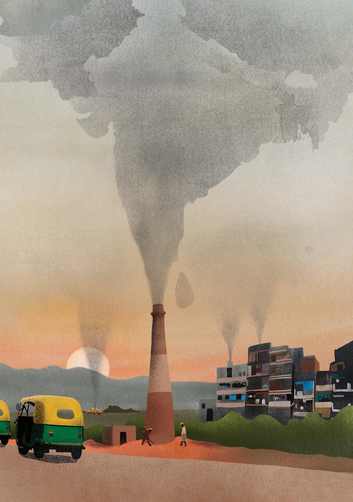
Cover illustration: © Reyes Work. Further permission required for reuse.
Cover design: Bill Pragluski, Critical Stages, LLC.
Library of Congress Control Number: 2023907856
South Asia is a global hotspot of air pollution, home to 37 of the 40 most polluted cities in the world. Some 60 percent of its population lives in heavily polluted areas where levels of dust particles exceed the least stringent World Health Organization (WHO) air quality standard. This air pollution is responsible for chronic respiratory disease and more than 2 million premature deaths a year in the region.
Dust particles can travel hundreds of kilometers, crossing municipal, state, and even national boundaries. For example, about 30 percent of air pollution in the Indian state of Punjab comes from neighboring Pakistan. Further east, an estimated 30 percent of pollution in Bangladesh’s largest cities originates in India due to the predominant wind direction from the northwest to the southeast.
This study finds that it is impossible to improve air quality to healthy levels using the city-by-city approach prevalent across South Asia today. For example, even if Delhi, the most polluted capital city in the world, were to fully implement all technically feasible air pollution control measures by 2030, the city would still not meet the WHO Air Quality Interim Target 1 if neighboring states and countries continue to follow their current policies. This is because the inflow of pollution from these states and bordering countries accounts for more than 50 percent of air particulate matter in Delhi. The same is true in many other cities, and in their surrounding rural areas as well. Only through cooperation at the province, state, and regional levels can South Asia hope to beat air pollution.
Current localized efforts to fight air pollution are not only falling short but are often focused on the most expensive abatement options. Cities in South Asia focus on air pollution emanating from power generation and motorized traffic, which is visible and politically salient. But this approach forgoes much cheaper abatement opportunities in agriculture, small firms, and solid waste management— many in peripheral areas adjacent to cities. This study uses an atmospheric model to simulate the effectiveness of a wide range of technological solutions to reduce air pollution, and by incorporating interregional links, allows us to analyze the benefits of acting together. The findings clearly demonstrate that coordinated solutions are more effective and, at the same time, cheaper.
While air pollution abatement will thus require bold political commitment and upfront investments, the economic benefits far outweigh the costs. In the full coordination scenario mentioned above, more than 750,000 lives would be saved annually, at a cost of just US$7,600 per life saved.
Other direct economic benefits from lower air pollution include reduced health expenditures and increased workplace productivity.
The following measures could facilitate cooperation across local and national administrative boundaries:
• Start with better data. South Asian countries could collaborate to install monitors at critical points throughout an airshed to generate credible scientific data and work together to build the institutional capacity to analyze them. This has been done in other parts of the world, including ASEAN countries, China, Europe, and the United States.
• Once the monitoring systems have been created, countries could establish joint airshed targets to track emissions within and across countries and encourage the adoption of cost-effective solutions. Joint efforts could involve sharing experiences in tackling key sources of air pollution in South Asia, including household burning of biomass fuel, brick kilns and ovens, burning of agricultural residue, and open burning of municipal waste, as well as sources of secondary particulate matter such as fertilizer, vehicle emissions, and large industry stacks.
• With good tracking mechanisms and joint targets in place, the region could begin to mainstream air quality in the economy by establishing emissions trading schemes so that cleaner and greener technologies become more competitive. The city of Surat in Gujarat, India, reduced particulate matter emissions by 24 percent through an innovative local emissions trading scheme. Much more would be possible if such schemes were extended across an airshed.
We take one breath every three seconds—38,000 breaths per day. Clean air is essential for our health, and tackling air pollution is imperative for passing on a better world to future generations. As people across South Asia demand cleaner air, their leaders will need to work together to deliver results.
This study was conducted with wide consultation with governments, nongovernmental organizations, and research and academic institutes in the region, and their contributions are gratefully acknowledged.
Martin Raiser Vice President South Asia Region The World BankThis report was prepared by a team led by Muthukumara Mani under the guidance of Hans Timmer (Chief Economist) and Martin Raiser (Vice President) of the South Asia Region of the World Bank. The core team members include Zara Ali, Ahmad Imran Aslam, Adanna Chukwuma, Martin Heger, Michael Norton, Jostein Nygard, Md. Shamemmur Rahman, Isabel Maria Ramos Tellez, Utkarsh Saxena, Siddharth Sharma, Nadia Sharmin, Aiga Stokenberga, Michael Toman, and Margaret Triyana. The team was supported in the modeling work by a team from the International Institute for Applied Systems Analysis (IIASA) that included Markus Amann and Wolfgang Schöpp (former staff), and Jens Borken-Kleefeld, Adriana Gomez-Sanabria, Chris Heyes, Gregor Kiesewetter, Zbigniew Klimont, Pallav Purohit, Parul Srivastava, and Fabian Wagner. Additional support was provided by Maureen Cropper, Bjorn Larsen, and Yongjoon Park.
The team greatly benefited from insightful comments and guidance from internal peer reviewers— Yewande Aramide Awe, Carter Brandon, and Ernesto Sanchez-Triana. The team is also grateful to other colleagues from the World Bank for their thoughtful comments and suggestions at various stages, most notably Pawan Bali, Christophe Crepin, Cecile Fruman, Elena Karaban, Magda Lovei, Janet Minatelli, Nicholas Muller, Urvashi Narain, Lynne Sherburne-Benz, Zoe Leiyu Xie, Yinan Zhang, and André Zuber.
The team thanks Diana Ya-Wai Chung, Elena Karaban, Mehreen Arshad Sheikh, and Adnan Javaid Siddiqi for guidance and support on the communication and dissemination strategy. Rana Al-Gazzaz provided critical support to the production, communication, and dissemination of this report. William Shaw provided editorial guidance. Peter Milne and Bart Ullstein provided excellent editorial support. The team also thanks Neelam Chowdhry and Ahmad Khalid Afridi for administrative support.
The team gratefully acknowledges timely financial support from the Program for Asia Resilience to Climate Change Trust Fund, a regional Trust Fund financed by the UK Foreign, Commonwealth, and Development Office on regional cooperation on climate change. The team would like to thank participants in various regional and national workshops and consultative meetings.
In producing this report, the World Bank emphasizes that air pollution initiatives and projects shall respect the sovereignty of the countries involved, and it notes that findings and conclusions in the report may not reflect the views of individual countries or their acceptance.
South Asians are exposed to extremely unhealthy levels of ambient air pollution, especially in densely populated, poor areas. Piecemeal approaches to reducing air pollution are unlikely to work since air pollution freely crosses boundaries. This report presents the following findings and discusses their importance for mitigating air pollution in the region:
• South Asia is home to 9 of the world’s 10 cities with the worst air pollution, which causes an estimated 2 million premature deaths across the region each year and results in significant economic costs.
• The report finds that concentrations of fine particulate matter such as soot and small dust (PM2.5) in some of the region’s most densely populated and poor areas are up to 20 times higher than what the World Health Organization (WHO) considers healthy (5 micrograms per cubic meter of air [μg/m 3]).
• Exposure to such extreme air pollution has impacts ranging from stunting and reduced cognitive development in children to respiratory infections and chronic and debilitating diseases.
• Current policy measures, even if fully implemented, will be only partially successful in reducing PM2.5 concentrations across South Asia.
• Air pollution travels long distances— crossing municipal, state, and national boundaries—and gets trapped in large “airsheds” that are shaped by climatology and geography.
• Large industries, power plants, and vehicles are dominant sources of air pollution around the world, but in South Asia, other sources make substantial additional contributions. These sources include combustion of solid fuel for cooking and heating, emissions from small industries such as brick kilns, burning of municipal and agricultural waste, and human cremation.
• Curbing air pollution requires not only tackling its specific sources but also close coordination among countries. Regional cooperation can be used to help implement cost-effective joint strategies that leverage the interdependent nature of air quality.
• The report identifies six major airsheds in South Asia where spatial interdependence in air quality is high. Particulate matter in each airshed comes from various sources and locations; for example, less than half the air pollution in South Asia’s major cities is produced within those cities.
• The report analyzes four scenarios for reducing air pollution with varying degrees of policy implementation and cooperation among countries. The most cost-effective scenario, which calls for full coordination between airsheds, would cut the average exposure to PM 2.5 in South Asia to 30 μg/m³ at a cost of US$278 million per μg/m 3 of reduced exposure, and would save more than 750,000 lives annually.
Though progress has been made in legislation and planning for air quality management, South Asia is not on track to reach even modest WHO targets. This report offers a three-phased road map to achieving clean air in an economically feasible manner in South Asia:
• Phase 1: The conditions for airshedwide coordination are set by expanding the monitoring of air pollution beyond the big cities, sharing data with the public, creating or strengthening credible scientific institutes that analyze airsheds, and taking a whole-of-government approach.
• Phase 2: Abatement interventions are broadened beyond the traditional targets of power plants, large factories, and transportation. During this phase, major progress can be made in reducing air pollution from agriculture, solid waste management, cookstoves, brick kilns, and small firms. At the same time, airshedwide standards can be introduced.
• Phase 3: Economic incentives are fine-tuned to enable private sector solutions, to address distributional impacts, and to exploit synergies with climate change policies. In this phase, trading of emission permits can also be introduced to optimize abatement across jurisdictions and firms.
South Asia is home to 9 out of the world’s 10 cities with the worst air pollution. South Asians are exposed to extremely unhealthy levels of ambient air pollution, especially in densely populated, poor areas. The World Health Organization’s (WHO’s) Air Quality Guidelines recommend that concentrations of PM2.5—small dust or soot particles in the air measuring 2.5 microns or less in width—should not exceed an annual average of 5 micrograms per cubic meter (μg/m3). In South Asia, however, nearly 60 percent of the population lives in areas where concentrations of PM2.5 exceed an annual mean of 35 μg/m3. On the densely populated Indo-Gangetic Plain, the level (100 μg/m3 in several locations) is more than 20 times what the WHO considers healthy.
Ambient air pollution is a public health crisis for South Asia, not only imposing high economic costs but also causing an estimated 2 million premature deaths each year. The health impacts of air pollution range from respiratory infections to chronic diseases, and from serious discomfort to morbidity and premature mortality. These effects drive up health care costs, lower productive capacity, and result in lost days worked.
Some of the main causes of air pollution in South Asia are unique to the region. Sources of air pollution that are less important in other parts of the world make substantial additional contributions to the pollution load in South Asia. These sources include solid fuel combustion in the residential sector for cooking and heating; small industries, including brick kilns; the burning of high-emission solid fuel; the current management practices of municipal waste, including the burning of plastics; the inefficient application of mineral fertilizer; fireworks; and human cremation. Significant air pollution in South Asia also emanates from agriculture, including through the generation of secondary particulate matter in the form of ammonia (NH₃) emissions from imbalanced fertilizer use and livestock manure that reacts with nitrogen oxides (NOx) and sulfur dioxide (SO₂) gases from energy, industry, and transportation sources. In the western part of South Asia, natural sources—such as dust, organic compounds from plants, sea salt, and forest fires—are a significant source of air pollution.
Controlling ambient air pollution is difficult without a better understanding of the activities that emit particulate matter and how emissions travel across locations. Air pollution travels long distances
within South Asia, crossing municipal, state, and national boundaries, depending on wind, climatology, and cloud chemistry. At any given location, PM2.5 in ambient air originates from several upwind sources extending over several hundred kilometers. This is especially true on and around the IndoGangetic Plain. For example, nearly 25 percent of the fine particulate matter to which residents of the city of Patna, India, are exposed has its origin in a neighboring state. In many cities—such as Dhaka, Bangladesh; Kathmandu, Nepal; and Colombo, Sri Lanka—only one-third of the air pollution originates within the city.
This report identifies six major airsheds in South Asia where spatial interdependence in air quality is high (map ES.1). Although air pollution travels far in South Asia, it is not uniformly dispersed over the continent. Instead, it gets trapped in large “airsheds” that are shaped by climatology
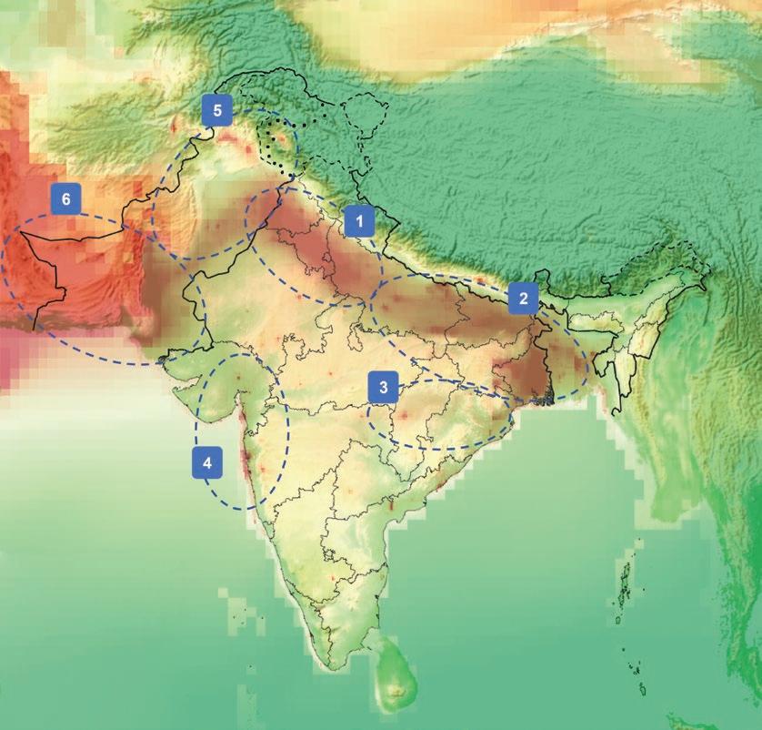
and geography. The six major airsheds in South Asia where spatial interdependence in air quality is high, as identified by the modeling exercise, are (1) the West/Central Indo-Gangetic Plain: Punjab (Pakistan), Punjab (India), Haryana, part of Rajasthan, Chandigarh, Delhi, and Uttar Pradesh; (2) the Central/Eastern Indo-Gangetic Plain: Bihar, West Bengal, Jharkhand, and Bangladesh; (3) Middle India 1: Odisha and Chhattisgarh; (4) Middle India 2: eastern Gujarat and western Maharashtra; (5) the Northern/Central Indus River Plain: Pakistan and part of Afghanistan; and (6) the Southern Indus Plain and further west: South Pakistan and western Afghanistan, extending into the eastern portion of the Islamic Republic of Iran.
This report uses a detailed geospatial model to quantify particulate matter emissions and how they disperse in the atmosphere. The Greenhouse Gas and Air Pollution Interactions and Synergies model used in this report computes the annual averages of PM2.5 concentrations to which residents of every state or province (hereafter referred to as “regions”) of South Asia are exposed. It also computes PM2.5 exposure at the city level and determines the place and the sector of origin of this ambient air pollution in each region and city.
The report shows that current policy measures will be only partially successful in reducing PM 2.5 concentrations across South Asia, even if fully implemented. The report’s model estimates that air quality policy measures in place as of 2018 can have a significant impact on the trajectory of air pollution in South Asia, if fully implemented and effectively enforced. For example, primary fine particulate matter (such as soot and mineral dust) would decline by 4 percent rather than grow by 12 percent between 2018 and 2030, regionwide. But large parts of South Asia—accounting for about two-thirds of its total population—will still miss the least-ambitious WHO Air Quality Interim Target 1 of 35 µg/m³ concentration.
Even if all technically feasible measures were fully implemented, parts of South Asia would still not be able to meet WHO Air Quality Interim Target 1 on their own by 2030 because of the spatial interdependence of air quality. Suppose the Delhi National Capital Territory (NCT) were to fully implement all technically feasible air pollution control measures by 2030, while other parts of South Asia continued to follow current policies. This report’s model predicts that the Delhi NCT area would still not meet the WHO Air Quality Interim Target 1 because the inflow of pollution from other regions and from natural sources already exceeds 35 µg/m³. The Delhi NCT would, however, meet the WHO Air Quality Interim Target 1 if other parts of South Asia also adopted all feasible measures, as is the case with many other cities in South Asia, especially those on the Indo-Gangetic Plain.
Accounting for the interdependence in air quality within airsheds in South Asia is necessary when weighing alternative pathways for pollution control. The report analyzes four alternative pathways (hereafter referred to as “scenarios”) for reducing air pollution in South Asia (table ES.1). These scenarios vary in the ambition of their air pollution targets and the degree to which their strategies for achieving those targets provide for regional coordination.
Pollution control scenarios that do not leverage spatial interdependence in air quality are relatively expensive. Scenario 1, which scales up measures already in place in parts of South Asia to other regions, would reduce average PM2.5 exposure in South Asia in 2030 to about 37 µg/m³. This is a bigger reduction than that achieved by full implementation of 2018 policies because all regions would undertake a common set of pollution control measures. Scenario 2, which entails full implementation of all technically feasible emissions controls everywhere across South Asia, would cut average PM2.5 exposure in South Asia in 2030 to 17 µg/m³. Not surprisingly, this would result in the biggest reduction among all four scenarios. However, this scenario is also the most expensive one because it uses all feasible measures regardless of their cost: its annual cost per µg/m³ of reduced exposure is US$2.6 billion.
Scenario 1: Ad hoc selection of measures
• Mean population exposure is reduced to 37 µg/m³
• Scaling-up of measures that are currently used in parts of South Asia to all its regions
• Each region acts independently
Scenario 3: Compliance with WHO Interim Target 1 everywhere in South Asia
• In all regions, mean population exposure is reduced to 35 µg/m³
• Regions cooperate to the extent they are contributing to pollution hotspots
Scenario 2: Maximum technically feasible emissions reductions
• Mean population exposure is reduced to 17 µg/m³
• Full implementation of all technical emissions controls that are available on the world market
• No regional coordination
Scenario 4: Toward the next lower WHO Interim Target
• In each region, reduce PM2.5 exposure to 90% of the gap with the next lower WHO Interim Target
• Full coordination across regions to maximize costeffectiveness
Focusing on the hotspots while leveraging the spatial interdependence of air pollution between hotspots and their upwind areas (Scenario 3) would reduce the mean exposure in South Asia to 26 μg/m³. The approach underlying this scenario reduces costs significantly by replacing excessively costly measures at hotspots with more cost-effective measures in areas upwind of hotspots, with an estimated cost of US$780 million per μg/m3 of reduced exposure. Thus, this scenario would achieve a significantly greater reduction in air pollution than Scenario 1, but at a comparable cost.
By cutting exposure toward the next lower WHO Interim Target in each region with full coordination across regions, the mean exposure in South Asia would decline to 30 μg/m³ in a cost-effective manner. Under Scenario 4, in which each region cuts exposure to 90 percent of the gap with the next lower WHO Interim Target, while fully leveraging spatial interdependence, the mean exposure in South Asia would decline to 30 μ g/m³. The approach followed in this scenario is the most cost-effective, at US$278 million per μg/m3 of reduced exposure. This result is achieved because the scenario uses the least-cost combination of measures within airsheds: it avoids implementing costly measures at one location if the same impact can be achieved by a less costly action at another location in the same airshed.
Scenario 4 also leverages sectoral differentiation to improve the cost-benefit ratio of pollution control measures. Compared with Scenario 2, where all technically feasible measures are implemented, Scenario 4 leans more heavily on lower-cost options in the household sector with cleaner cookstoves and liquefied petroleum gas solutions and the control of secondary particulate matter, particularly through agricultural sector interventions such as balanced fertilizer application and manure management. The scenario also focuses on managing the burning of municipal waste. See figure ES.1 for an illustration of the outcomes of each scenario.
Regional cooperation could thus help realize cost-effective joint air pollution control strategies that leverage spatial interdependence in air quality. As the scenario modeling shows, if regions within South Asia were to work toward their air quality targets independently of each other, those with relatively limited options for improving air quality may be forced to undertake costly measures. Meanwhile, those with good options for improving air quality may not exercise some of those options because they do not account for the benefits to other regions from doing so.
Regional coordination could also help break deadlocks in policy action by increasing certainty about the payoffs from different policy scenarios. Because of the spatial interdependence in air
quality, each region’s expectations about future air quality if it were to take certain pollution control measures depend on expectations about actions taken by others. Policy makers may choose to delay costly actions because of uncertainty about future air quality. Regional coordination may help speed up action by firming up expectations about future air quality.
Steps to reduce ambient and household air pollution could significantly reduce premature deaths. The four scenarios outlined in the report involve policies to reduce emissions of ambient PM2.5 from stationary and mobile sources—such as power plants, factories, and motor vehicles—and also reduce the number of households burning solid fuels. Deaths avoided in 2030 from reductions in PM2.5 according to the four scenarios range from 276,000 to 1,270,000, and the average cost per life saved for each scenario varies from US$7,600 to US$68,000. The impacts of these reductions in PM2.5 on premature mortality are measured from baseline values of ambient and household air pollution in 2030.
The effectiveness of air pollution control policies in reducing premature deaths varies greatly across policies and within regions. Under Scenario 1, which reflects traditional air pollution control measures, 276,000 premature deaths are avoided, but the scenario only reduces baseline deaths caused by air pollution in Nepal, Pakistan, and Sri Lanka by 3–4 percent. The policies are slightly more effective in India, reducing deaths by 15 percent on the Indo-Gangetic Plain and, on average, by 16 percent in the rest of India. In Bangladesh, deaths are reduced by 7 percent. These policies come at a cost per life saved of US$38,000. In contrast, the policies in Scenario 2 are much more effective, reducing premature deaths by 1,270,000, or 55–85 percent across countries. However, the average cost per life saved by these policies is US$68,000.
The analysis shows that Scenario 4, with a PM2.5 level of 30 μg/m3, has the lowest per capita cost of averting premature deaths and the highest benefit-to-cost ratio for morbidities. Policies under this scenario save more lives—more than 750,000 annually—than policies in Scenario 3, and at a much lower cost per life saved, at US$7,600, or only 11 percent of the cost under Scenario 2. Reductions in baseline deaths resulting from these lower-cost policies show geographical variation. Specifically, the reductions in Sri Lanka and non-Indo-Gangetic Plain India are larger than the reductions from the set of policies in Scenario 3, although the reduction in deaths is 10–15 percentage points lower in other regions of South Asia. The lower cost per life saved by policies under Scenario 4 is achieved by relying on reductions in the percentage of households burning solid fuel, which should also benefit more women and children.
Though progress has been made in legislation and planning for air quality management (AQM), South Asia is not on track to reach even the modest WHO Interim Target 1. That target of 35 μg/m³ is still seven times the concentration that the WHO considers healthy. The reason for insufficient progress is that, currently, the focus of interventions is almost completely on mitigating pollution generated within cities. Most countries in South Asia have imposed varying emissions standards for vehicles and have mandated low-NOx burners for power plants and filters for some large industrial boilers. To achieve more progress—and more cost-effective progress—the policy focus should broaden into other sectors, especially small manufacturing, agriculture, residential cooking, and waste management, which are important sources of air pollution in South Asia. Along with the broadening of the sectoral focus, coordination of abatement activities within larger areas (within the airsheds) is needed.
This report shows that optimal solutions for achieving clean air are economically feasible in South Asia, but that the implementation of these policies is challenging. The report demonstrates that the economic benefits of these optimal policies exceed the economic costs by a large margin. However, implementation of these policies requires coordination that provides incentives for cooperation across different jurisdictions and coordination between nations because airsheds do not recognize national borders. Under the predominant wind direction from the northwest to the southeast, 30 percent of the air pollution in the Indian state of Punjab comes from Punjab Province in Pakistan and, on average, 30 percent of the air pollution in the largest cities of Bangladesh (Dhaka, Chittagong, and Khulna) originates in India. During parts of the year, substantial pollution flows in the other direction across borders. Optimal AQM also requires changes in the behavior of millions of farmers; small enterprises, including small-scale brick kilns; and households. Such behavioral change is not easy to achieve in practice. The journey toward that optimal solution is best guided by the following road map, which breaks down the journey into three phases, each consisting of three steps.
Cost-effective AQM requires more comprehensive monitoring, including outside cities; enhanced scientific capacity; a shared knowledge base; and strong cooperation between governments.
• Emissions inventories are currently incomplete in South Asia. South Asia should move toward a comprehensive, unified inventory for the region that represents the full range of relevant emissions sources instead of relying on each city or state to develop its own methodology.
• Transparency and accessibility are important components of a monitoring system. The accessibility of data on unified platforms is critical to the sharing of knowledge and the building of trust across jurisdictions. Public awareness of air quality data can also help build support for AQM.
• Monitoring systems need to be maintained and updated on an ongoing basis. Technology will continuously improve, perhaps changing which policy choices are most cost-effective or even rendering some policy action obsolete.
• Scientific capacity in South Asia is currently well developed in atmospheric science, but it is still relatively underdeveloped when it comes to capturing the region-specific sources of air pollution. Further development of analytical capacity should include research into health impacts and analysis of economic incentives and behavioral adjustments. All these areas suffer from a knowledge gap regarding the influence of specific circumstances in South Asia.
• Scientific capacity should not be centralized, but rather distributed across the region. To enhance the credibility and salience of scientific information among the stakeholders of airsheds, and to ensure more equal representation and ownership across countries and jurisdictions, a South Asia–wide scientific community on AQM should facilitate communication between experts across administrative boundaries and develop a scientific consensus on critical issues.
• The capacity of ministries of the environment must be strengthened. These ministries have the principal mandate to manage air quality programs, but they have neither the financial resources nor the staff required for the needed coordination of environmental policies in agriculture, energy, industry, rural development, transportation, and urban development.
• A strong and central technical role of ministries of the environment should be complemented with a whole-of-government approach. AQM can have far-reaching consequences for other policy areas, from energy and climate policy to growth strategy and distributional policies. The report shows how synergies between AQM and climate policies can be exploited. The report also shows that there is significant overlap between local air quality and poverty in South Asia, and that abatement efforts can have distributional impacts. To ensure consistency with the broader development strategy, a whole-of-government approach to AQM is needed.
Airshedwide AQM will automatically include low-cost abatement of more sources of air pollution. Once the focus broadens beyond cities, other emissions, which are especially important in South Asia, can be reduced. These include emissions from solid fuel use in households, from brick kilns and ovens in other small industries, from agriculture, and from open burning of solid municipal waste.
• Cleaner cookstoves are cost-effective, but implementation challenges remain. Despite the effectiveness of clean cookstoves in improving health, three main challenges to long-term adoption remain: (1) initial and maintenance costs, (2) knowledge and beliefs, and (3) compatibility with end users. These challenges imply that economic support and information, in addition to adequate price signals, are key to achieving the adoption of clean fuel technology by mostly poor, rural households.
• Burning of fields results in high seasonal peaks in air pollution throughout airsheds. Recent evidence from India shows that cash transfers as payments for ecosystem services can reduce agricultural burning by up to 80 percent.
• Subsidies for fertilizers, another cause of air pollution, should be reconsidered. Other interventions can also successfully lower fertilizer use without compromising productivity. For example, Bangladesh’s simple rule-of-thumb training using colored leaf charts lowered fertilizer use by 8 percent without compromising yields.
• Large-scale intensive livestock operations can prevent emissions through the scrubbing of ventilated air both into and out of animal housing areas. Various types of air purification systems exist, including combination filters that remove more than one pollutant. Abatement measures for animals not contained within housing include a switch to low-nitrogen feed, covered storage of manure, and application of manure on farms with technology designed to reduce ammonia emissions.
• Less-polluting and more viable brick kiln technologies are available but slow in being adopted. Many brick kilns in South Asia are very small units using old technologies, with inefficient combustion of coal and agricultural waste. Existing kilns can be converted to improved “zigzag” kilns that produce less emissions and are more efficient in brick production. However, the adoption rate of zig-zag kilns remains low, implying that behavioral change requires more than price incentives.
• Municipal waste management is one of the most cost-effective potential interventions in the region. In many cities in South Asia, no waste collection is performed, and even in cities with high collection rates, segregation of waste and recycling hardly occurs. Recycling, controlled incineration, composting of biodegradable waste, and managed landfills not only reduce air pollution but also generate revenues, for example, by recovering precious or rare earth metals from electronic components.
In the long run, pricing of externalities through taxation or tradable emissions permits should play a central role in AQM. In the short run, mandated emissions standards, authorized filters or technologies, and bans on certain activities are the most effective methods for reducing air pollution. However, these methods come with disadvantages. Emissions standards reduce emissions per unit of economic activity, but they do not curb the total amount of polluting activity. Emissions standards also do not incentivize the private sector to develop technologies that reduce pollution to levels below mandated standards. If pollution has a cost in the form of a tax or the price of an emissions permit, total emissions are reduced more, and innovation is stimulated. With these economic incentives, private and public funds to reduce air pollution are more easily mobilized.
Step
• Taxation of activities that release pollutants will make cleaner technologies more competitive. Likewise, subsidies can encourage the use of clean industries and technologies that do not harm air quality. Currently, most examples of taxes on air pollutants are found in developed economies. These taxes target primarily greenhouse gases or cover only one type of source (typically, large power plants or large firms in high-polluting industries). However, developing countries are increasingly experimenting with direct taxes on pollutants. China has an environmental protection tax on PM2.5 precursors (SO₂, NOx, and soot). Mexico imposed a carbon tax in 2014.
It applies to carbon emissions from all sectors and covers all fossil fuels except natural gas. In October 2021, Indonesia passed a law to introduce a carbon tax on coal-fired power plants.
• Tradable emissions permits can have significant advantages. An airshedwide system of tradable emissions permits gives firms throughout the airshed more flexibility to adjust their emissions and incentives to innovate, and it automatically provides pecuniary compensation across jurisdictions for abatement efforts. Most examples of these permit markets are in developed countries, but similar programs are now being piloted or under consideration in China, Mexico, Thailand, and Türkiye.
• Recent evidence from a pilot of permit trading in India is encouraging. The state of Gujarat recently introduced emissions-permit trading among 317 high-polluting plants. A critical precondition for this plan was the installation of a robust monitoring system in the participating firms. The pilot has been evaluated through a randomized control trial, which shows that it reduced emissions significantly and at low cost relative to the existing command-and-control regulation.
• An important advantage of the use of economic incentives is that they can mobilize funds from the private and public sectors for clean technologies. When the negative externalities of air pollution are incorporated into the price of technologies, the private sector finds investing in clean technologies to be profitable. The larger the area that imposes taxes, the easier it is for the private sector to invest at scale. Revenues from taxes on pollutants or from sales of emissions permits generate the fiscal space to create public funds that support abatement activities. Such funds can play an important role in enticing cooperation within an airshed across jurisdictions.
• The synergies between reductions in air pollution and climate change policies can help mobilize international funds. Strong synergies are found between meeting cleaner air targets and meeting commitments to reduce greenhouse gas emissions. Those synergies can mobilize international funds that can support AQM. Some of these funds come from multilateral development banks, scaling up existing programs that link financing to the achievement of air quality improvement targets.
Achieving cleaner air in South Asia in a cost-effective way is possible, but the road ahead is not an easy one. The analysis in this report shows that, from a technical point of view, direct economic gains from better air quality exceed the abatement costs needed to reduce air pollution. However, achieving these optimal solutions is not easy. It requires the building of better monitoring systems, more scientific capacity, and better coordination between governments. It requires behavioral change by farmers, small firms, and households. It requires experiments with the greening of tax systems and with tradable emissions permits. International experience has to be fine-tuned to the specific conditions in South Asia. It requires cross-border coordination in South Asia, which is far from straightforward, but the time is now to put conditions in place for such cross-border cooperation and the time is now to travel the road to cleaner air. The rewards of advancing on the road are high given that the economic and social costs of a lack of progress are hard to overestimate.
AAP ambient air pollution
AQM air quality management
AQMD air-quality-management district
ASEAN Association of Southeast Asian Nations
CO2 carbon dioxide
μg/m3 cubic meter
ETS emission trading system
GAINS Greenhouse Gas and Air Pollution Interactions and Synergies, model developed by IIASA
GDP gross domestic product
HAP household air pollution
IGP Indo-Gangetic Plain
IHME Institute for Health Metrics and Evaluation
IIASA International Institute for Applied Systems Analysis
IV instrumental variable
LPG liquefied petroleum gas
NCT National Capital Territory (Delhi, India)
NH3 ammonia
NMVOC nonmethane volatile organic compounds
NOx nitrogen oxides
PAF population-attributable fraction
PM2.5 fine particulate matter (e.g., small dust or soot particles) in the air measuring 2.5 microns or less in width
PPM par ts per million
SO2 sulfur dioxide
WHO World Health Organization
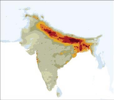
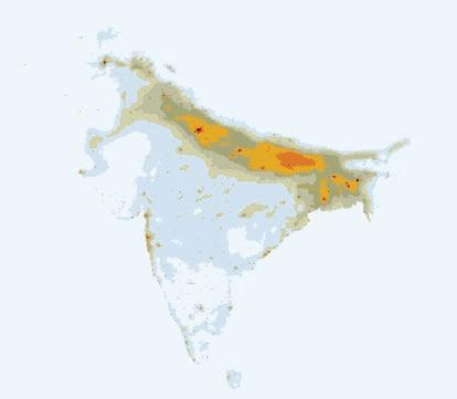
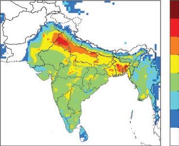
South Asia suffers from extreme air pollution. Of the world’s 10 cities with the most severe air pollution, 9 are in South Asia. In the northern part of the region, which has a high proportion of poor households, the average annual concentration of fine particulate matter (PM2.5) is about 16 times the maximum that the World Health Organization considers healthy (map 1.1). In addition to high ambient air pollution, poor households also experience high levels of indoor air pollution, caused by the use of solid fuel for cooking and heating.
The exposure to extreme air pollution has severe health impacts. Current air pollution is estimated to cause more than 2 million premature deaths each year in South Asia. PM 2.5 is now also understood to be an important causative factor in many noncommunicable health risks. For newborns, it has been associated with low birthweight and premature birth. For children, it can lead to asthma, stunting, and reduced cognitive development, with lifelong consequences. In adults, PM2.5 is associated with chronic obstructive lung disease, ischemic heart disease, lower respiratory infections, lung cancer, strokes, and type 2 diabetes. For the elderly, a correlation with dementia has been established.
Air pollution comes with economic costs. Increased morbidity raises health care costs and reduces the number of days worked per person. Stunting leads to lower productivity later in life. Firms and skilled workers might choose not to locate in areas with severe air pollution (Lozano-Gracia and Soppelsa 2019). Potentially, factories could be temporarily closed or traffic could be temporarily limited during periods of peak pollution.
South Asian countries have made strides in strengthening air quality management programs, but more work is needed. A wave of policy responses have been introduced in recent years to combat air pollution, including the draft Bangladesh Clean Air Act, India’s National Clean Air Programme, and the National Electric Vehicles Policy in Pakistan. These recent policy changes will allow economies to grow without corresponding increases in air pollution. Further measures beyond these decoupling efforts will, however, be necessary for South Asian countries to reduce air pollution.
To effectively reduce air pollution, cooperation across jurisdictions is needed. Less than half of the air pollution in the major cities of South Asia is produced within the cities themselves.


At the same time, air pollution that originates in cities spreads well beyond city borders. Air pollution is transported over long distances, and then trapped in large “airsheds” shaped by climatology and geography. Because the air pollution in a location within an airshed arrives from different locations both within and outside that airshed, the sources of air pollution are diverse, ranging from power plants, large factories, and traffic, to agricultural emissions, waste burning, brick kilns, and cooking. Figure 1.1 shows the variety of sources in the Delhi National Capital Territory (NCT), and the significant contributions from locations beyond the Delhi NCT. Much of the focus of air pollution

Others
Livestock, fertilizer
Agriculture residue burning
Municipal waste
Mobile sources
Residential
Small industries
High stacks
dust, sea salt
PPM others
PPM livestock, fertilizer
PPM agriculture residue burining
PPM municipal waste
PPM mobile sources
PPM residential
PPM small industries
PPM high stacks
Secondary PM
Soil dust, sea salt
management in South Asia has been at a city level and on a few major polluters within the city. For more effective air quality management, coordination within airsheds is needed, and the focus should widen to a broader group of polluters.
This study is organized as follows: Chapter 2 provides a picture of the various sources of air pollution in South Asia and how these sources interact and form airsheds. Chapter 3 presents various alternative scenarios for cost-effective pollution control measures and studies the costs of these scenarios as compared with existing legislation. The health impacts arising from these four scenarios are calculated in chapter 4, along with the estimated economic benefits of reductions in air pollution. Chapter 5 discusses policy recommendations, including the development of airshed-scale management strategies. Such strategies will require more information and transparent incentives for cooperation across jurisdictions.
Kummu, Matti, Maija Taka, and Joseph H. A. Guillaume. 2020. Data from Gridded global datasets for Gross Domestic Product and Human Development Index over 1990–2015, Dryad, Dataset. Accessed November 14, 2022, https://doi.org/10.5061/dryad.dk1j0.
Lozano-Gracia, Nancy, and Maria E. Soppelsa. 2019. “Pollution and City Competitiveness: A Descriptive Analysis.” Policy Research Working Paper 8740, World Bank, Washington, DC.
This study uses a series of well-established scientific tools and methods that provide a holistic perspective on air quality in South Asia, and explores the costs and benefits of different policy interventions intended to reduce air pollution in the region. As a starting point for the subsequent strategic analyses, a comprehensive assessment of the current state of air quality in South Asia reveals the most important sources of pollution and how these sources affect air quality in cities and regions (provinces and states) throughout South Asia.
The Greenhouse Gas and Air Pollution Interactions and Synergies (GAINS) model is used to provide a holistic perspective on the chain of air pollution in the region (Amann et al. 2011).1 Starting from the socioeconomic drivers, the GAINS model quantifies emissions and their dispersion in the atmosphere and estimates their multiple impacts on air quality and human health. Importantly, the model assesses the improvements offered by about 2,000 proven measures to reduce emissions, estimates their costs, and quantifies their side effects on greenhouse gas emissions. The cost-effectiveness analysis of the model identifies packages of measures that deliver exogenously specified policy targets on air quality or greenhouse gas emissions (or both) at least cost (figure 2.1). Details of the modeling exercise are given in annex 2A.
Some of the key aspects of the modeling approach follow:
• To inform efforts to protect public health in an economically effective way, the modeling uses the annual average population-weighted mean exposure to ambient fine particulate matter (PM2.5) as the central metric. It should be noted, however, that mean population exposure is lower than the highest concentrations measured at hotspots, which are relevant for establishing compliance with ambient air quality standards.
• The model computes grid average PM 2.5 concentrations throughout the domain at a 10 × 10–k ilometer spatial resolution. With these data, the mean population exposure over the entire population in an administrative region can be computed. It is necessary, however, to ensure that the modeled data are validated with data from various monitoring stations (figure 2.2) to ensure good predictability of future scenarios.
control options: ~2000 measures, co-control of 10 air pollutants and 6 greenhouse gases
Source: International Institute for Applied Systems Analysis.
Note: GAINS = Greenhouse Gas and Air Pollution Interactions and Synergies.
Average Fine Particulate Concentrations by Source for 10 × 10–Kilometer Grid Cells Compared with Observations from Monitoring Stations Located within the Grid Cells in Delhi NCT, 2018
FIGURE
Sources: Calculations using GAINS model developed by the International Institute for Applied Systems Analysis; India CPCB 2020.
Note: NCT = National Capital Territory; PM2.5 (µg/m³) = fine particulate matter measured in micrograms per cubic meter.
Beyond their contributions to human exposure to PM2.5 in ambient air, some emissions sources cause additional health impacts through exposure in indoor environments. Although the study addresses the management of pollution in ambient air, several emissions sources cause additional health impacts through the exposure pathway in indoor environments. Severe health impacts are estimated
to result from exposure to emissions from the combustion of solid fuel for cooking and heating in households without proper ventilation, adding to the high health burden from exposure to pollution from these sources in ambient air. The quantification of the interplay of household and ambient exposure is discussed further in chapter 4, which provides estimates of the total health impacts from all sources that generate ambient air pollution.
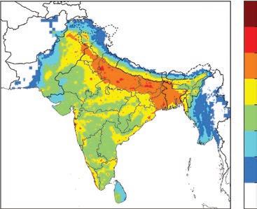
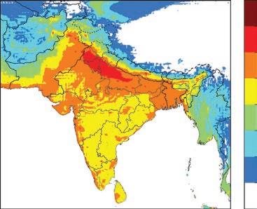
Although the ambient levels of PM2.5 differ considerably across South Asia, average annual concentrations exceed the World Health Organization’s (WHO’s) Air Quality Guidelines of 5 micrograms per cubic meter by a wide margin throughout South Asia. Generally, the highest levels occur on the Indo-Gangetic Plain, where annual mean concentrations exceed the WHO guidelines by a factor of 20 or more. Further concentration peaks appear in many cities, as well as in desert areas. In contrast, concentrations are much lower in the southern part of the South Asia region, although there they also surpass the WHO guidelines by a wide margin.
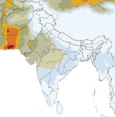
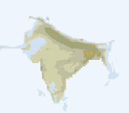
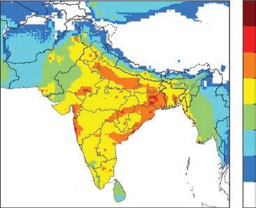
In some parts of South Asia, rather large contributions to PM 2.5, in both relative and absolute terms, originate from natural sources, including from soil dust in arid regions (map 2.1, panel a). Some of the natural sources of air pollution are organic compounds from plants and sea salt. Other natural sources are released during such catastrophes as volcanic eruptions and forest fires. The importance of natural sources that cannot be immediately influenced by policy interventions has to be kept in mind when setting policy targets for total PM2.5 concentrations in ambient air, either in absolute terms such as in ambient air quality standards, or relative ones, for example, percentage reductions of total PM2.5 concentrations relative to a base year.
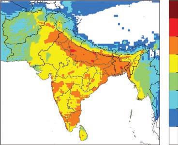
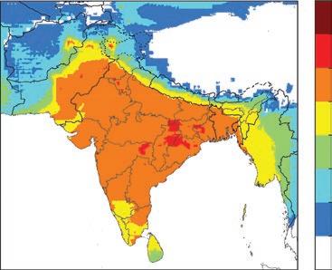
Throughout South Asia, secondary PM2.5 particles, formed through chemical reactions in the atmosphere from gaseous precursor emissions, account for a sizable fraction of total PM2.5 concentrations in ambient air. Fine particulate matter in ambient air is composed of so-called primary particles,

such as soot and mineral dust, which are directly emitted, as well as secondary particles and aerosols, which are formed in the atmosphere in chemical processes from precursor emissions of sulfur dioxide (SO 2 ), nitrogen oxides (NOx), ammonia (NH 3 ), and nonmethane volatile organic compounds (NMVOC). Over large areas in South Asia, such secondary particles and aerosols account for a sizable fraction of total PM2.5 in ambient air, often exceeding the contributions of primary particles from anthropogenic sources (map 2.2). This has major implications for air quality management (AQM): effective strategies need to address the full range of emissions, including those of precursors of secondary particles and aerosols. Strategies focused on primary particles and aerosols can achieve only limited reductions of total PM 2.5 concentrations in ambient air and are unlikely to deliver costeffective improvements because they neglect potential low-cost options for limiting emissions of precursors of secondary PM2.5
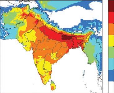
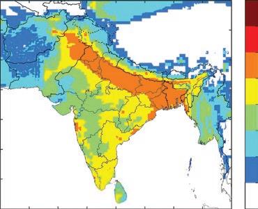
In addition to emissions sources that are common throughout the world, certain activities specific to South Asia contribute large amounts of PM 2.5 in ambient air. As in many other regions of the world, power generation, large-scale industries, and mobile sources are responsible for significant shares of total PM2.5 concentrations in South Asia, together often exceeding the WHO guidelines value. However, there are other sources that are less important in other world regions that make substantial additional contributions to the pollution load in South Asia, on top of the sources that are most prevalent across the world. These sources include, among others, solid fuel combustion in the residential sector for cooking and heating; small industries, including brick kilns; the burning of high-emissions solid fuel; current management practices for municipal waste in the region, including the burning of plastics; inefficient application of mineral fertilizer; fireworks; and human cremation. Contributions of these source categories to total PM 2.5 concentrations in ambient air in South Asia are shown in map 2.3. As a result, policy interventions that focus only on emissions sources that are prominent across the world would have a limited impact
(figure continued next page)
MAP 2.3 Concentrations of Fine Particulate Matter in Ambient Air Originating from Key Emissions Sectors, 2018 (continued)
Source: Calculations using GAINS model developed by the International Institute for Applied Systems Analysis.
Note: PM2.5 (µg/m³) = fine particulate matter measured in micrograms per cubic meter.
FIGURE 2.3 Contributions to Population-Weighted Fine Particulate Matter Exposure in Cities on the Indo-Gangetic Plain by Source, 2018
Others
Manure and fertilizer
Agricultural residue burning
Municipal waste
Mobile sources
Residential and commercial
Small industry (including brick kilns)
Power plants and large industry
Soil dust and sea salt
Source: Calculations using GAINS model developed by the International Institute for Applied Systems Analysis.
Note: PM2.5 (µg/m³) = fine particulate matter measured in micrograms per cubic meter.
on total PM2.5 concentrations in the South Asia region because they miss the large contributions caused by South Asia–specific pollution sources.
Because of the diversity of sources that contribute to PM2.5 in ambient air in South Asia, particulate matter at any given receptor site needs to be traced to many different sectors. Although quantitative shares differ across cities and provinces or states because of local topographic, meteorological, and economic factors, no one sector—except for isolated pollution hotspots—can be identified as the single source responsible for the majority of PM 2.5 at any given location (figures 2.3 to 2.5).
Because of the multisectoral character of the sources of air pollution in South Asia, effective AQM, in addition to the sources that have been the focus of past efforts, that is, road transportation and large point sources, will need to involve other sectors that are important in specific subregions, such as household energy uses, small industries (for example, brick kilns), waste management, and agricultural activities.
Wind can carry PM2.5 particles in the atmosphere through the air for several hundred to a few thousand kilometers before they are deposited on the surface. Thus, at any given location, PM2.5 in ambient air originates from a wide range of upwind sources extending over several hundred kilometers. Equally, emissions from any given source will be carried over similar distances and
Others
Manure and fertilizer
Agricultural residue burning
Municipal waste
Mobile sources
Residential and commercial
Small industry (including brick kilns)
Power plants and large industry
Soil dust and sea salt
Others
Manure and fertilizer
Agricultural residue burning
Municipal waste
Mobile sources
Residential and commercial
Small industry (including brick kilns)
Power plants and large industry
Soil dust and sea salt
affect air quality over large downwind areas. Figures 2.6 to 2.8 reveal the origin of ambient PM 2.5 concentrations at specific locations. Especially on the Indo-Gangetic Plain, with its high large-scale emissions density, a rather small share of population-weighted PM2.5 exposure comes from lowlevel sources such as road traffic, the residential sector, and waste management in the same city, whereas the majority of PM2.5 exposure originates from other sources in the same province or state. In other areas where outside pollution levels are generally lower, a larger share of PM2.5 pollution in cities originates from local sources.
Low-level sources in the city
Same state
Neighboring states
Rest of India
Other countries
Natural soil dust
Low-level sources in the city
Same state
Neighboring states
Rest of India
Other countries
Natural soil dust
Effective AQM in South Asia therefore needs to balance measures across sectors and coordinate interventions with other upwind regions. Given the variety of contributing sources, effective solutions need balanced combinations of measures across sectors and regions, and should prioritize those measures that achieve air quality improvements at relatively low cost. The support of various stakeholder groups may be facilitated by a robust and shared knowledge base on emissions sources and their consequences for air quality.
Although the long-range transport of pollution requires regional coordination, effective AQM should also tailor solutions to local conditions. The share of local sources of ambient PM2.5 varies across South Asia, depending on topography, meteorology, the intensity and spatial patterns of emissions, and the size of the administrative regions. Figures 2.9 to 2.14 compare sources across the Indo-Gangetic Plain city of Patna, India; Chennai, India; Dhaka, Bangladesh; Kathmandu, Nepal; Rawalpindi, Pakistan; and Colombo, Sri Lanka. As can be seen, the sources vary significantly within and across the major cities in South Asia.
Low-level sources in the city
Same province or division
Rest of the country
Other countries
Natural soil dust
Other
Livestock, fertilizer
Agricultural residue burning
Municipal waste
Mobile sources
Residential
Small industries
High stacks
Soil dust, sea salt
(figure continued next page)
FIGURE
b. Primary and secondary PM, Patna
PPM other
PPM livestock, fertilizer
PPM agricultural residue burning
PPM municipal waste
PPM mobile sources
PPM residential
PPM small industries
PPM high stacks
Secondary PM
Soil dust, sea salt
Allocations of Population Exposure to Total Fine Particulate Matter and Primary versus Secondary Fine Particulate Matter in Patna, Bihar State, India, 2018 (continued) From
Source: Calculations using GAINS model developed by the International Institute for Applied Systems Analysis.
Note: PM = particulate matter; PM2.5 (µg/m³) = fine particulate matter measured in micrograms per cubic meter; PPM = parts per million.
FIGURE
Allocations of Population Exposure to Total Fine Particulate Matter and Primary versus Secondary Fine Particulate Matter in Chennai, Tamil Nadu State, India, 2018
a.
Other
Livestock, fertilizer
Agricultural residue burning Municipal waste
Mobile sources
Residential Small industries
High stacks
Soil dust, sea salt
(figure continued next page)
PPM livestock, fertilizer
PPM agricultural residue burning
PPM municipal waste
PPM mobile sources
PPM residential
PPM small industries
PPM high stacks
Secondary PM
Soil dust, sea salt
Source: Calculations using GAINS model developed by the International Institute for Applied Systems Analysis. Note: PM = particulate matter; PM2.5 (µg/m³) = fine particulate matter measured in micrograms per cubic meter; PPM = parts per million.
Other
Livestock, fertilizer
Agricultural residue burning
Municipal waste
Mobile sources
Residential
Small industries
High stacks
Soil dust, sea salt
(figure continued next page)
PPM other
PPM livestock, fertilizer
PPM agricultural residue burning
PPM municipal waste
PPM mobile sources
PPM residential
PPM small industries
PPM high stacks
Secondary PM
Soil dust, sea salt From
other divisions
same division
the city
Source: Calculations using GAINS model developed by the International Institute for Applied Systems Analysis. Note: PM = particulate matter; PM2.5 (µg/m³) = fine particulate matter measured in micrograms per cubic meter; PPM = parts per million.
Other
Livestock, fertilizer
Agricultural residue burning
Municipal waste
Mobile sources
Residential
Small industries
High stacks
Soil dust, sea salt
(figure continued next page)
PPM other
PPM livestock, fertilizer
PPM agricultural residue burning
PPM municipal waste
PPM mobile sources
PPM residential
PPM small industries
PPM high stacks
Secondary PM
Soil dust, sea salt
Source: Calculations using GAINS model developed by the International Institute for Applied Systems Analysis. Note: PM = particulate matter; PM2.5 (µg/m³) = fine particulate matter measured in micrograms per cubic meter; PPM = parts per million.
Other
Livestock, fertilizer
Agricultural residue burning
Municipal waste
Mobile sources
Residential
Small industries
High stacks
Soil dust, sea salt
FIGURE 2.13 Source Allocations of Population Exposure to Total Fine Particulate Matter and Primary versus Secondary Fine Particulate Matter in Rawalpindi, Pakistan, 2018 (continued)
b. Primary and secondary PM, Rawalpindi
PPM other
PPM livestock, fertilizer
PPM agricultural residue burning
PPM municipal waste
PPM mobile sources
PPM residential
PPM small industries
PPM high stacks
Secondary PM
Soil dust, sea salt
From natural sources
From other countries
From other provinces
From the same province
From the city
Source: Calculations using GAINS model developed by the International Institute for Applied Systems Analysis.
Note: PM = particulate matter; PM2.5 (µg/m³) = fine particulate matter measured in micrograms per cubic meter; PPM = parts per million.
FIGURE 2.14 Source Allocations of Population Exposure to Total Fine Particulate Matter and Primary versus Secondary Fine Particulate Matter in Colombo, Sri Lanka, 2018
a. Total sector contributions, Colombo
From natural sources From other countries From same division From the city
Other
Livestock, fertilizer
Agricultural residue burning
Municipal waste
Mobile sources
Residential
Small industries
High stacks
Soil dust, sea salt
(figure continued next page)
PPM other
PPM livestock, fertilizer
PPM agricultural residue burning
PPM municipal waste
PPM mobile sources
PPM residential
PPM small industries
PPM high stacks
Secondary PM
Soil dust, sea salt
The strong spatial interconnections between emissions sources in the South Asia region limit the ability of single cities, states, and provinces to achieve steep reductions in pollution concentrations on their own, even if they could eliminate all emissions within their own territory. This situation is not, however, unique to South Asia. Useful approaches have been developed in other parts of the world to coordinate AQM among different jurisdictions. In particular, the airshed concept emphasizes the common responsibility for a shared resource—that is, the air mass in each region—and facilitates coordinated but differentiated response strategies that achieve effective air quality improvements while respecting heterogeneity in the ability of different regions to act.
An airshed can be defined as a region that shares a common flow of air, which may become uniformly polluted and stagnant. Air quality within an airshed will largely depend on pollution sources within it. The extension of an airshed is strongly determined by the spatial distribution and intensity of emissions sources, as well as the typical patterns of pollution transportation in the atmosphere, which depend on local geography, meteorology, and climatic conditions.
Because the formation of secondary particles and the transporting of primary and secondary particles take place over large geographic areas, airsheds can extend over several hundred kilometers, well beyond the boundaries of cities.
The need for airshedwide coordination emerges particularly for the urban areas of South Asia, in which a high share of PM2.5 pollution in ambient air is imported from outside the area. In most cases, cities alone cannot achieve steep reductions in pollution, even if they could eliminate all emissions within their own territory.2 Given the prevailing high concentrations in many urban agglomerations in South Asia, coordination between administrative regions that constitute common airsheds, e s pecially between cities and the surrounding states or provinces, will be indispensable in moving toward the WHO Air Quality Interim Targets, and especially for doing so in a cost-effective manner.
To explore potential candidate airsheds in South Asia, this study applied a two-step approach that considers the following physical features (note that political considerations are not addressed here):
1. O verlay pollution concentration maps 3 —yearly PM 2.5 concentrations in 10 × 10–k ilometer grid cells—on elevation maps to define where concentrations are trapped within the topography.
2. Determine PM 2.5 transportation patterns between source regions within the airshed compared with PM 2.5 transportation patterns inside and outside the airshed.
This approach revealed six priority regions (map 2.4):
1. West/Central Indo-Gangetic Plain: Punjab (Pakistan), Punjab (India), Haryana, part of Rajasthan, Chandigarh, Delhi, and Uttar Pradesh
2. Central/Eastern Indo-Gangetic Plain: Bihar, West Bengal, Jharkhand, and Bangladesh
MAP 2.4 Six Major Airsheds in South Asia Based on Fine Particle Concentrations, Topography, and Fine Particle Transportation between Source Regions
3. Middle India 1: Odisha and Chhattisgarh
4. Middle India 2: eastern Gujarat and western Maharashtra
5. Northern/Central Indus River Plain: Pakistan and part of Afghanistan
6. Southern Indus Plain and further west: South Pakistan and western Afghanistan, extending into eastern Islamic Republic of Iran.
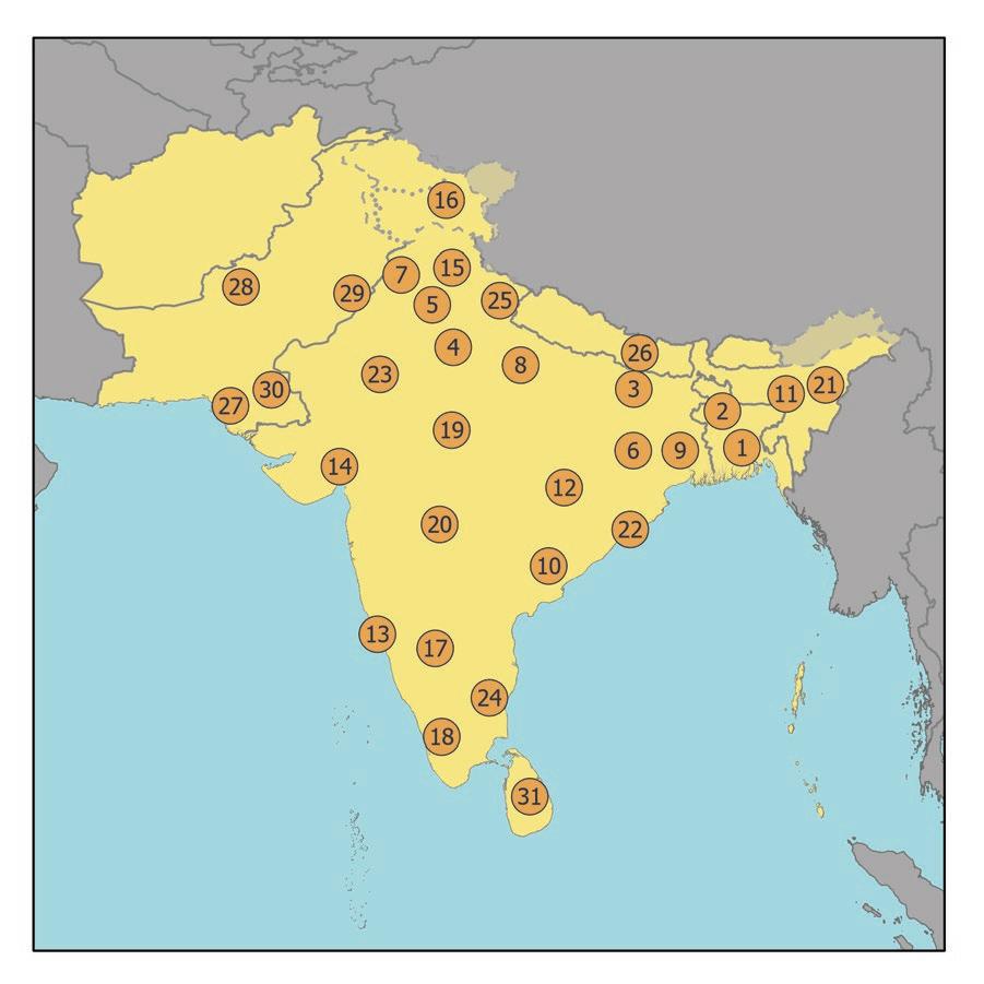
To capture the diversity across South Asia, the GAINS model implementation for this study distinguished 31 emissions source regions (individual states and provinces of large countries). The impacts of their emissions on regional air quality were computed for more than 500 individual cities as well as for rural areas at a spatial resolution of about 50 × 50 kilometers (0.5 × 0.5 degrees).
Although air pollution has a wide range of negative impacts on human health, agricultural crops, and natural ecosystems, this analysis focuses on the most harmful pollutant to human health, PM2.5 It does not assess additional threats to human health and vegetation caused by ground-level ozone or to biodiversity from excess nitrogen deposits, or damage to sensitive terrestrial and aquatic ecosystems caused by acid deposits.
Any effective clean air strategy will vary in approach based on the context of each country or city, as well as its capacity to develop and implement measures. There is no uniform policy prescription for air quality that is applicable to all countries and regions; such an approach would neither be possible nor desirable for a problem that is so diverse in local circumstances.
The modeling studies reviewed in the report were conducted using data on economic activities, emissions, and ambient concentrations of the relevant pollutants in Bangladesh, India, Nepal, Pakistan, and Sri Lanka. For Bangladesh, India, and Pakistan, the analysis focused on 29 subnational regions, covering individual states or divisions or aggregates of these. These subregions are used for scientific convenience only and have no official or administrative significance.
The analysis presented in this report attributes changes in air quality to sources both within and outside each of the 31 study regions (map 2A.1). The regions are used for scientific convenience only; but by studying which regions are affected by others, it is possible to suggest which regions would benefit most from cooperation. Thus, the regions may be considered the building blocks for potential airsheds, which may be made up of two or more of the study regions.
This report developed a preliminary methodology for delineating airsheds in South Asia, which required taking many factors into account, including physical geography together with economic and political considerations, and involved developing both pollution concentration maps and PM2.5 transportation patterns.
The analysis for South Asia is fed by numerous local data sources supplemented by relevant international information that has been obtained under comparable conditions. To capture the specific characteristics of the region, implementation of the GAINS framework for South Asia drew on a wide range of national data, including, among others, published statistics on socioeconomic characteristics, fuel consumption, industrial and agricultural activities, and the transportation and waste management sectors.
This report developed coherent emissions inventories for all precursor emissions of PM2.5 in South Asia. For each of the 31 regions, the study compiled emissions inventories of the relevant air
(table continued next page)
Rajasthan
Uttar
Other
Whole
Karachi
Khyber Pakhtunkhwa and Balochistan
Punjab (Pakistan)
Sindh 31
Sri Lanka
Whole country
pollutants: primary PM2.5, SO2, NOx, NH3, NMVOCs, and short-lived climate pollutants. Estimates were developed for 2015 and 2018, considering the effectiveness of applied emissions control measures. Priority was given to local measurements, and data gaps were filled by information from international studies conducted for similar socioeconomic and technological conditions.
The spatial patterns of PM2.5 and its precursor emissions were estimated at a 0.5 × 0.5–degree longitude–latitude resolution, based on relevant proxy variables updated from Klimont et al. (2017). These estimates rely on the most recent updates of data on plant locations, remote sensing of open biomass burning, and waste statistics that were originally developed within the Global Energy Assessment project (GEA 2012). For the residential and transportation sectors, finer resolved emissions distribution maps were developed at a 10 × 10–kilometer resolution, using fine-scale gridded population data and road maps. Natural emissions are based on estimates used by the European Monitoring and Evaluation Programme (Simpson et al. 2012) and GEOS-Chem (van Donkelaar et al. 2019) atmospheric chemical and transportation models.
Air quality is assessed over all South Asia at a spatial resolution of 10 × 10 kilometers and compared with available monitoring data. The fine-scale emissions inventory serves as an input for the calculation of PM2.5 concentrations in ambient air across South Asia. Using the well-established European Monitoring and Evaluation Programme atmospheric chemical-transportation model (Simpson et al. 2012), total annual mean concentrations of PM2.5 were computed for the 200 largest cities, while concentrations in rural areas were estimated at a 10 × 10–kilometer resolution. These calculations combined the fine-scale dispersion characteristics of primary PM2.5 emissions, which lead to steep
gradients around emissions sources, with the formation of secondary particles and the long-range transport of PM2.5 in the atmosphere. These were computed at a 0.5 × 0.5–degree longitude–latitude, which is about a 50 × 50–kilometer resolution. Calculations were conducted at hourly intervals for meteorological data sets for 2015 and 2018.
After validation of the computed concentrations against available observations, the dispersion model was used to distill the spatial dispersion pattern of low- and high-level emissions sources of primary PM2.5, SO2, NOx, NH3, and NMVOC for each South Asian emissions source region. Assuming constant meteorological conditions for 2018, these source-receptor relationships were then used to estimate concentration fields for different emissions patterns, for example, those resulting from the application of emissions controls in the future.
Although public attention and legislative AQM focuses on episodic concentration peaks at pollution hotspots, the maximization of public health benefits is better served by a focus on population exposure. In many cases, public attention on air pollution focuses on the most polluted places, comparing measured concentrations against national ambient air quality standards. This approach is aligned with the prevailing legal frameworks for AQM, which prescribe compliance with national ambient air quality standards throughout the entire territory, and thereby in the most polluted places. Observed concentration peaks—for example, at curbsides in busy streets—are, however, not necessarily the best metric for protecting public health, given that they are only loosely related to long-term exposure of the entire population, which has been identified as the most powerful predictor of the adverse health impacts from air pollution.
1. The GAINS model is an analytical framework for assessing future potential outcomes and costs for reducing air pollution impacts on human health and the environment while simultaneously mitigating climate change through reduced greenhouse gas emissions. It explores synergies and trade-offs in cost-effective emissions control strategies to maximize benefits across multiple scales.
2. However, the specific conditions in several areas of South Asia call for airshed management approaches that include multiple states, provinces, and even countries. The delineation of airsheds must encompass many factors, including physical geography, as well as economic and political considerations, and their definition inevitably involves subjective judgments.
3. PM2.5 concentration maps were generated from the GAINS model by the International Institute for Applied Systems Analysis (IIASA); topographic maps were made by the World Bank. The map overlay was made by the World Bank project team.
Amann, M., I. Bertok, J. Borken-Kleefeld, J. Cofala, C. Heyes, L. Höglund-Isaksson, Zbigniew Klimont, et al. 2011. “Cost-Effective Control of Air Quality and Greenhouse Gases in Europe: Modeling and Policy Applications.” Environmental Modelling and Software 26 (12): 1489–501. https://doi .org/10.1016/j.envsoft.2011.07.012
GEA. 2012. Global Energy Assessment—Toward a Sustainable Future . Cambridge: Cambridge University Press; and Laxenburg, Austria: International Institute for Applied Systems Analysis. www.globalenergyassessment.org
India CPCB (Central Pollution Control Board). 2020. National Ambient Air Quality Monitoring Programme (NAMP) Data. Ministry of Environment and Forests, Government of India. http://www.cpcbenvis.nic.in/air_quality_data.html.
Klimont, Z., K. Kupiainen, C. Heyes, P. Purohit, J. Cofala, P. Rafaj, J. Borken-Kleefeld, and W. Schöpp. 2017. “Global Anthropogenic Emissions of Particulate Matter Including Black Carbon.” Atmospheric Chemistry and Physics 17 (14): 8681–723. https://doi.org/10.5194/acp-17-8681-2017.
Simpson, D., A. Benedictow, H. Berge, R. Bergström, L. D. Emberson, H. Fagerli, C. R. Flechard, et al. 2012. “The EMEP MSC-W Chemical Transport Model—Technical Description.” Atmospheric Chemistry and Physics 12: 7825–65. https:// doi.org/10.5194/acp-12-7825–2012.
van Donkelaar, A., R. V. Martin, C. Li, and R. T. Burnett. 2019. “Regional Estimates of Chemical Composition of Fine Particulate Matter Using a Combined Geoscience-Statistical Method with Information from Satellites, Models, and Monitors.” Environmental Science and Technology 53 (5): 2595–611. https://doi.org/10.1021/acs.est.8b06392.
The cost-effectiveness of alternative approaches for further air quality improvements varies, and the most cost-effective scenarios are those that explicitly consider transboundary pollution. This chapter considers four pollution control scenarios that differ based on the level of ambition, the rationale for prioritizing efforts, and the degree of coordination across jurisdictions. These four scenarios range from one that only scales up current efforts to one that envisions use of the maximum technically feasible measures for reducing air pollution.
As a starting point, a baseline projection for 2030 is first developed, revealing the pivotal importance of the full implementation and enforcement of recently adopted air quality legislation. Many factors other than legislation will change the relative contribution of the various economic sectors to emissions, including new technology, population growth, growing urbanization, and economic development. This baseline projection assumes continued population and economic growth, with a doubling of per-person income between 2018 and 2030. Economic structural changes and programs for enhanced energy efficiency will reduce the energy intensity of GDP, such that total primary energy consumption will grow less than total GDP. Reduced poverty and recent policies on access to clean fuels will reduce the number of households using solid biomass by 60 percent. In contrast, vehicle kilometrage closely follows the income trend (figure 3.1).
Air quality policies and measures adopted by South Asian governments so far will help decouple emissions trends from GDP growth, but the extent will depend on enforcement of this recent legislation. Compared with the assumed increase in GDP by 2030, the emissions controls already implemented, together with structural economic changes and energy policies, will moderate further growth of fine particulate matter (PM 2.5) precursor emissions. Since 2015, governments have introduced additional legislation, but it has yet to be fully implemented. If fully implemented and effectively enforced, these new measures would deliver much lower emissions: primary PM 2.5 would decline by 4 percent rather than grow by 12 percent; sulfur dioxide would decline by 43 percent instead of increasing by 39 percent; and growth in nitrogen oxides would decline to 10 percent from 46 percent. However, ammonia emissions would not be affected because there is no relevant legislation (figure 3.2). The large difference between the 2015 and 2018 legislation cases highlights the
Sources: Calculations using GAINS model developed by the International Institute for Applied Systems Analysis; World Bank World Development Indicators.
Avoided through economic restructuring and 2015 pollution controls
Potential reduction from full implementation of 2018 legislation
Baseline projection assumed in this report 2018 emissions
Source: Calculations using GAINS model developed by the International Institute for Applied Systems Analysis.
Note: Emissions would increase by 160 percent absent interventions. The dark green bars represent the avoided exposure in 2030 resulting from implementation of the 2015 legislation package. The orange bars show additional reductions in exposure that could be achieved by the full and efficient implementation of the additional policies and measures in the 2018 package. The blue bars show the expected 2030 emissions with the implementation of the 2015 and 2018 legislation. PM2.5 = fine particulate matter; GDP = gross domestic product.
importance of strict enforcement of current policies and measures, and illustrates the potential gains from the effective implementation of the recent legislation. These policies and measures will not, however, be sufficient to reduce PM 2.5 concentrations throughout the region to meet the World Health Organization (WHO) Air Quality Interim Target 1 of 35 micrograms per cubic meter (μg/m³) in large parts of South Asia (map 3.1). The effective enforcement of recent pollution control legislation will affect the margin of uncertainty around future
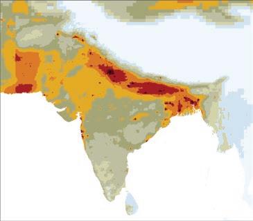
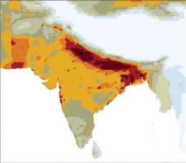

FIGURE
2030
by the full and efficient implementation of the additional policies and measures of the 2018 package. The gray diamonds denote the mean population exposure in 2018 and the gray bars show the contribution from natural sources (soil dust and sea salt). PM2.5 = fine particulate matter; µg/m³ = micrograms per cubic meter.
air quality. Not only could the recently adopted legislation compensate for increased emissions from the steep increase in economic activity that is projected, but it could also deliver effective reductions in ambient PM2.5 concentrations in many areas.
The envisaged structural changes in the economy, together with the already-implemented emissions controls, will prevent significant deterioration from current levels. Whether they will reduce current population exposure (the gray diamonds in figure 3.3), however, depends on the effectiveness of implementation (the blue bars). Thus, in areas with high concentrations of PM2.5 today, such as the Indo-Gangetic Plain and urban agglomerations in other regions, mean that population exposure will remain far above WHO Interim Target 1 of 35 μg/m³, and even with the introduction of the latest measures, about two-thirds of the population in South Asia will remain exposed to PM 2.5 concentrations above this target level.
Given the limited air quality improvements that can be expected from the recent legislation, additional air quality measures and cost implications are examined for four alternative approaches to air quality management (AQM) in South Asia:
• The ad hoc selection of measures scenario assesses a scaling-up of the measures that are currently in place in parts of South Asia to the whole region. Following current widespread thinking in the region, the main focus is on the power sector, large-scale industry, and road transportation. Costeffectiveness receives less attention, and measures are often decided upon with no regard for air quality interactions from other territories.
• The maximum technically feasible emissions reduction scenario explores the range of air quality improvements that could be achieved by 2030 from full implementation of all technical emissions controls that are currently available on the world market—irrespective of cost. New technologies are introduced only through new investment, with no allowances made for premature scrapping of the existing capital stock.
• The compliance with WHO Interim Target 1 scenario provides a more targeted approach; AQM focuses on pollution hotspots in South Asia and brings mean population exposure to PM2.5 in each region into compliance with WHO Interim Target 1 of 35 μg/m3. Addressing the long-range transport of pollution to the most-polluted areas requires regional coordination, and measures in other regions are selected based on their cost-effectiveness.
• The toward the next lower WHO Interim Target scenario seeks cost-effective cuts in harmful population exposure to PM2.5 through a common but differentiated approach that is coordinated across South Asia. With a long-term aim of moving toward the next lower WHO Interim Target for PM2.5, measures are selected such that, by 2030, the present difference in mean population exposure to the next lower WHO Interim Target level in each region falls by 90 percent.1 Measures are chosen based on their cost-effectiveness and, where necessary, coordinated with neighboring regions.
Beyond the 2018 air quality legislation, the scenarios (table 3.1) outline the significant scope for further air quality improvements that could be achieved through additional measures. By 2030, implementation of the maximum technically feasible emissions reductions scenario throughout South Asia could bring mean population exposures to PM2.5 in each region distinguished in this analysis below WHO Interim Target 1. This reduction is indicated by the orange bars in figure 3.4, star ting from the exposure levels that emerge from compliance with the 2018 legislation. In this case, average population exposure in South Asia could be reduced by about two-thirds, from about 50 μg/m³ in 2018 to 17 μg/m³ in 2030. Residual exposure originates from natural sources (the dark green bars in figure 3.4) and from emissions that cannot be removed by currently available technical measures. Importantly, several regions, especially on the Indo-Gangetic Plain and in urban agglomerations,
Scenario 1: Ad hoc selection of measures
• Mean population exposure is reduced to 37 µg/m³
• Scaling-up of measures that are currently used in parts of South Asia to all its regions
• Each region acts independently
Scenario 3: Compliance with WHO Interim Target 1 everywhere in South Asia
• In all regions, mean population exposure is reduced to 35 µg/m³
• Regions cooperate to the extent they are contributing to pollution hotspots
Scenario 2: Maximum technically feasible emissions reductions
• Mean population exposure is reduced to 17 µg/m³
• Full implementation of all technical emissions controls that are available on the world market
• No regional coordination
Scenario 4: Toward the next lower WHO Interim Target
• In each region, reduce PM2.5 exposure to 90% of the gap with the next lower WHO Interim Target
• Full coordination across regions to maximize costeffectiveness
cannot achieve WHO Interim Target 1 on their own, even if they implemented all technically feasible measures (indicated by the blue bars), because the inflow of pollution from outside regions and from natural sources already exceeds 35 μg/m³.
Without coordination, regions cannot reliably predict their future air quality. The long-range transport of pollution makes actual air quality improvements in a region dependent not only on local measures but also on measures taken in other areas. This is illustrated in figure 3.5, in which the orange bars indicate, for 2030, exposure reductions from the measures taken in the ad hoc selection of measures scenario within the same region. Obviously, benefits from the local measures account for only a minor share of the full potential and miss WHO Interim Target 1 by a wide margin in many regions. At the same time, however, regions will enjoy the spillover benefits from measures taken beyond their borders (the tan bars in figure 3.5), but the extent of these would, without regional coordination, remain unknown.2 Airshedwide coordination of measures enhances the effectiveness of AQM strategies. A lack of knowledge of the spillover impacts from measures in other regions within the same airshed will inevitably lead to costly AQM solutions because it prohibits selection of the most efficient measures to meet given air quality targets. Airshedwide coordination, despite its governance challenges, has proven to be a powerful mechanism in other regions of the world (for example, California in the United States, the European Union, and the Jing-Jin-Ji Metropolitan Region of China) for enhancing the economic efficiency of effort spent on AQM.
Indo-GangeticPlain
Other IndiaOther coun tries
2018
Improvements from the local measures taken in the ad hoc selection of measures scenario Possible further improvements from measures taken in other regions
Potent ial improvements from all local measures Potential improvements from all measures in all other regions
Two of the above-noted scenarios—compliance with WHO Interim Target 1 scenario and toward the next lower WHO Interim Target scenario—illustrate the power of coordinated approaches. In both cases, regions would cooperate to the extent necessary for achieving common air quality improvement targets through differentiated action such that, overall, the economic resources spent on pollution controls are minimized.
The two scenarios aim at different air quality targets and result in different distributions of air quality benefits and costs:
• Following conventional approaches, the compliance with WHO Interim Target 1 scenario prioritizes action in the most-polluted places by imposing a uniform target that should be met in all regions of South Asia. For convenience, WHO Interim Target 1 of 35 μg/m³ has been adopted for 2030. The ambient PM2.5 levels under this scenario are often lower than under the toward the next lower WHO Interim Target scenario, especially on the Indo-Gangetic Plain.
• In the toward the next lower WHO Interim Target scenario, all regions reduce their mean exposure levels gradually along the four WHO Interim Targets of 35, 25, 15, and 10 μ g/m³ toward the WHO guideline of 5 μ g/m³. This more innovative approach does not delay progress that could easily be made in less-polluted places until the air quality target becomes achievable in the more-polluted places. Most important, a more uniform distribution of air quality improvements delivers significantly higher health benefits to societies while harvesting gains from lowcost measures.
Because of their contrasting target-setting rationales, the four scenarios result in rather different distributions of air quality improvements (map 3.2). Most notably, in 2030, WHO Interim Target 1 appears achievable throughout South Asia, except in areas with high levels of pollution from natural sources. Local hotspots with exposures above 35 μg/m³ remain in the scenarios, even if the mean exposure in the region falls below this level.
The four AQM approaches differ not only in the amount and regional distribution of improvements, but also in their cost-effectiveness:
• As a benchmark, compliance with the 2018 legislation involves costs of about US$74 billion per year through 2030, or 1.4 percent of GDP annually. This reduces mean population exposure to PM2.5 in South Asia to about 47 μg/m³ in 2030, compared with 50.5 μg/m³ in 2018 (figure 3.6).
• Full implementation of all technically feasible emissions controls, as outlined in the maximum technically feasible emissions reduction scenario, would cut exposure in 2030 to 17 μg/m³, a reduction of two-thirds of 2018 levels, at a cost of US$86 billion per year, or 1.6 percent of GDP, on top of the cost of implementing the 2018 legislation. Expressed differently, the annual cost of reduced exposure per μg/m³ is US$2.6 billion.
• Scaling up the current emissions controls, as outlined in the ad hoc selection of measures scenario, would reduce mean exposure to 37 μg/m³, a reduction of about one-quarter of 2018 levels, at additional costs beyond those of the 2018 legislation of US$10.6 billion per year, or 0.20 percent of GDP annually through 2030.
• Focusing on the most-polluted areas by bringing down exposure everywhere below WHO Interim Target 1 of 35 μg/m3, as outlined in the compliance with WHO Interim Target 1 scenario, halves the mean exposure in South Asia to 26 μg/m³, as a result of the co-benefits of upwind measures at other locations. Additional costs increase to US$19 billion per year, or 0.35 percent of GDP annually through 2030. Interestingly, at a cost of US$780 million per μg/m³ of reduced exposure, the cost-effectiveness of these two last approaches is broadly similar.
• The most cost-effective air quality improvements emerge from a common but differentiated move toward the WHO Interim Targets, as outlined in the toward the next lower WHO Interim Target scenario. If each region were to cut exposure to below the next lower interim target, mean exposure in South Asia would decline to 30 μg/m³, a reduction of 40 percent of 2018 levels. Additional annual costs amount to US$5.7 billion per year, or 0.11 percent of GDP annually through 2030. Notably, costs of such an approach are 45 percent lower than those of the ad hoc selection of measures scenario, while it would deliver 70 percent higher reductions in total exposure in South Asia. At US$278 million per μg/m³ of reduced exposure, this approach is the most cost-effective.
The toward the next lower WHO Interim Target scenario maximizes cost-effectiveness by identifying the measures that deliver differentiated exposure targets at the least cost for each region. Although the analysis was carried out for each of the 31 study regions, figure 3.7 presents the impacts of individual measures on mean exposure levels in six aggregated areas: the IndoGangetic Plain, other regions of India, Bangladesh, Nepal, Pakistan, and Sri Lanka. The dark green bars indicate exposure improvements that will result from implementation of the 2018 legislation, the orange bars show exposure reductions from the cost-effective measures in the toward the next lower WHO Interim Target scenario, and the blue bars outline the scope for further improvements from measures that are not cost-e ffective in this scenario. Depending on the sector, further improvements that fall into the gray bars include more expensive clean cookstove variants, control of smaller units in the power sector, and the retrofitting of vehicles to meet the equivalent of the Euro-6 emissions standard.3
This shift in AQM strategies is also reflected in the costs that emerge of control measures in various sectors. Out of the total estimated cost of US$73 billion per year for implementation of the 2018
0102030405060708090100110120130
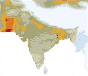
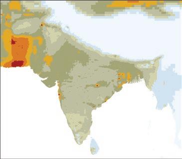
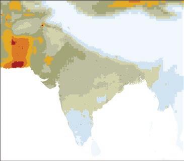
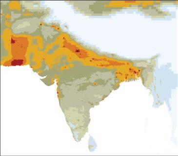

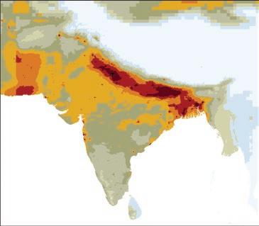
legislation across South Asia through 2030, the vast majority, US$55 billion, is for road transportation, followed by US$12 billion for emissions controls in the power sector (figure 3.8). Implementation of all additional measures that are technically feasible would require a further US$86 billion per year; additional controls for mobile sources, such as agricultural equipment, would consume 45 percent of these costs.
In contrast, additional costs in the toward the next lower WHO Interim Target scenario amount to only US$5.7 billion per year, of which about half is due to measures in the household sector. About 40 percent of the cost of additional measures is linked to further controls on mobile sources, power generation, and industry, which are already addressed in the 2018 legislation; and 10 percent emerges from the agriculture sector through, for example, measures to control agricultural residue burning, fertilizer application, and manure management.
The important two-way transporting of pollution across city limits, state boundaries, and even national borders becomes particularly relevant when considering cost-effective policy interventions to improve air quality without imposing excessive burdens on the economy. Especially in areas with high emissions density and topographic and meteorological conditions that include air exchange with other regions, a lack of knowledge about action in other regions makes it impossible to determine effective sets of measures to meet a given air quality target or to choose those measures that deliver the target at least cost. In the scenarios considered in this study, coordination across locations is the key feature that makes the toward the next lower WHO Interim Target scenario the most cost-effective. On the Indo-Gangetic Plain and in Bangladesh, about 40 percent of the exposure reductions emerge from action taken in other states or countries, and this share is even higher in other areas that benefit from action in the most-polluted places (figure 3.9).
Clean cooking and lighting
Municipal solid waste incineration
Trucks and buses
Power sector
Industrial SO2+NOx emissions
Steel and cement production
Fertilizer use
Municipal solid waste recycling
Nonroad mobile machinery
Vehicles—inspection and maintenance
Residentia l heating
Agricultural residue burning
Cars and two-wheelers
Other
Industrial PM2.5 emissions
Brick kiln s
Diesel generators
Solvents
Manure management
Gasoline stations
a. Indo-Gangetic Plain, India
Power sector
Clean cooking and lighting
Industrial SO2+NOx emissions
Municipal solid waste incineration
Trucks and buses
Steel and cement production
Industrial PM2.5 emission s
Residential heating
Agricultural residue burnin g
Brick kilns
Vehicles—inspection and maintenance
Cars and two-wheelers
Municipal solid waste recycling
Fertilizer use
Nonroad mobile machinery
Other
Manure management
Diesel generators
Solvents
b. Other regions, India
Clean cooking and lighting
Power sector
Agricultural residue burning
Municipal solid waste incineration
Trucks and buses
Industrial SO2+NOx emissions
Nonroad mobile machinery
Municipal solid waste recycling
Fertilizer use
Steel and cement production
Vehicles—inspection and maintenance
Residential heating
Industrial PM2.5 emissions
Brick kilns
Diesel generators
Cars and two-wheelers
Manure management Other
Solvents
Gasoline stations
Exposure reduction (µg/m³)
Exposure reduction (µg/m³)
c. Bangladesh d. Nepal
Clean cooking and lighting
Trucks and buses
Municipal solid waste incineration
Power sector
Vehicles—inspection and maintenance
Industrial SO2+NOx emissions
Municipal solid waste recycling
Agricultural residue burning
Steel and cement production
Fertilizer use
Nonroad mobile machinery
Diesel generators
Residential heating
Cars and two-wheelers
Brick kilns
Other
Manure management
Industrial PM2.5 emission s
Clean cooking and lighting
Municipal solid waste incineration
Power sector
Trucks and buses
Municipal solid waste recycling
Agricultural residue burning
Vehicles—inspection and maintenance
Cars and two-wheelers
Steel and cement production
Brick kilns
Fertilizer use
Industrial SO2+NOx emissions
Diesel generators
Residential heating
Nonroad mobile machinery
Industrial PM2.5 emissions
Exposure reduction (µg/m³)
Exposure reduction (µg/m³)
e. Pakistan f. Sri Lanka
Clean cooking and lighting
Industrial SO2+NOx emissions
Power sector
Trucks and buses
Municipal solid waste incineration
Vehicles—inspection and maintenance
Fertilizer use
Steel and cement production
Cars and two-wheelers
Municipal solid waste recycling
Industrial PM2.5 emission s
Residential heating
Nonroad mobile machinery
Manure management
Brick kilns
Other
Agricultural residue burnin g
Diesel generators
Exposure reduction (µg/m³)
Exposure reduction (µg/m³)
Source: Calculations using GAINS model developed by the International Institute for Applied Systems Analysis. Note: The orange bars indicate the cost-effective reductions from the measures in the toward the next lower WHO Interim Target scenario. Scales vary for each panel. Fine particulate concentrations (PM2.5 ) are in micrograms per cubic meter (µg/m 3 ). SO2+NOx = sulfur dioxide and nitrogen oxides; WHO = World Health Organization.
Source: Calculations using GAINS model developed by the International Institute for Applied Systems Analysis. Note: GDP = gross domestic product; WHO = World Health Organization.
FIGURE 3.9 Fine Particulate Matter Exposure Reductions in the Toward the Next Lower WHO Interim Target Scenario That Emerge from Measures Taken within a Region, Country, State, or Province, and from Measures Taken at Upwind Sources in Other Areas
Changes from measures in the same state or emissi on region
Changes from measures in other states on the IGP
Changes from measures in other regions in the same country
Changes from measures in other countries
Residual exposure from anthropogenic activities
Exposure from natural sources (soil dust)
Source: Calculations using GAINS model developed by the International Institute for Applied Systems Analysis. Note: IGP = Indo-Gangetic Plain; PM2.5 (µg/m³) = fine particulate matter measured in micrograms per cubic meter; WHO-IT1 = WHO Interim Target 1.
A systematic framework for air quality planning and management
Atmospheric CTM models, for example, EMEP, CMAQ, WRF-chem, AERMOD, CHIMERE, and others
Source: International Institute for Applied Systems Analysis.
Note: AERMOD = modeling system of the American Meteorological Society/Environmental Protection Agency Regulatory Model Improvement Committee; CHIMERE = a multiscale chemical-transportation model for atmospheric composition analysis and forecast; CMAQ = Community Multiscale Air Quality model; CTM = chemical-transportation model; EMEP = European Monitoring and Evaluation Programme; GAINS = Greenhouse Gas and Air Pollution Interactions and Synergies; PM2.5 = fine particulate matter; WRF-chem = Weather Research and Forecasting (WRF) model coupled with chemistry.
Proven tools for a systematic cost-effectiveness analysis of AQM are available, but more reliable data are needed to provide robust quantitative policy advice. The strong mutual connections between pollution inflows from upwind sources and outflows into downwind areas open opportunities for AQM to enhance cost-effectiveness by balancing measures across regions in such a way that cost savings and benefits from airshedwide coordination are maximized. The GAINS model has proven effective in shaping cost-effective airshed policies in China and Europe (figure 3.10) (Klaassen, Berglund, and Wagner 2005; Lu et al. 2019).
1. The WHO Air Quality Guidelines for mean annual concentrations of PM2.5 is 5 µg/m3. The WHO has established four interim targets toward the achievement of the guideline: Interim Target 1, 35 µg/m3; Interim Target 2, 25 µg/m3; Interim Target 3, 15 µg/m3; and Interim Target 4, 10 µg/m3. The 90 percent reduction would allow different regions to move toward different interim targets, depending on their 2018 pollution level.
2. Starting from the exposure following compliance with 2018 legislation (figure 3.5), the medium green bars indicate further possible improvements from implementation of all measures that could be taken within a region. The medium green bars show additional improvements that could result from measures taken in other regions. The dark green dots show exposure in 2018. The orange bars show improvements in exposure to fine particulate matter from the measures taken in the ad hoc selection
of measures scenario within the region, and the tan bars show possible further improvements from measures taken in other regions.
3. “Commission Regulation (EU) No 459/2012 of 29 May 2012 amending Regulation (EC) No 715/2007 of the European Parliament and of the Council and Commission Regulation (EC) No 692/2008 as regards emissions from light passenger and commercial vehicles (Euro 6) Text with EEA relevance” (https://eur-lex.europa.eu/legal-content/EN/TXT/?uri=celex%3A32012R0459).
Klaassen, Ger, Christer Berglund, and Fabian Wagner. 2005. “The GAINS Model for Greenhouse Gases— Version 1.0: Carbon Dioxide (CO2).” IIASA Interim Report IR-05-53. International Institute for Applied Systems Analysis, Laxenburg, Austria.
Lu, Zhenyu, Lin Huang, Jun Liu, Ying Zhou, Mindong Chen, and Jianlin Hu. 2019. “Carbon Dioxide Mitigation Co-Benefit Analysis of Energy-Related Measures in the Air Pollution Prevention and Control Action Plan in the Jing-Jin-Ji Region of China.” Resources, Conservation & Recycling: X 1: 100006. https://doi.org/10.1016/j.rcrx.2019.100006.
The health impacts of air pollution range from respiratory infections to chronic diseases, and from serious discomfort to morbidity and premature mortality. Acute and sustained exposure to household and ambient air pollution can affect people at each phase in their life cycle (figure 4.1). Exposure to air pollution in utero increases the probability of fetal loss, premature birth, and low birthweight. In early childhood, air pollution can cause respiratory infection and stunting (HeftNeal et al. 2022). These early-life health impacts often persist into adulthood (Almond and Currie 2011; Barker 1995; Currie et al. 2014). For older children, adults, and the elderly, exposure to air pollution increases the risk of respiratory infection. Air pollution also poses a risk to mental health (Chen, Oliva, and Zhang 2018). A significant correlation has been found between exposure to air pollution for adults and the elderly and the number of deaths caused by a multitude of noncommunicable diseases, including cardiopulmonary disease and type 2 diabetes, presumably because air pollution increases the likelihood of those diseases or it makes those diseases more likely to be fatal (Balakrishnan et al. 2019; Cohen et al. 2017; Murray et al. 2020). Although it is not easy to establish exact causes of diseases, several techniques have been used over the years to estimate the impact of both household air pollution and ambient air pollution. This research started with epidemiological studies using time series and cohort studies. More recently, quasi-experimental methods, such as difference-in- differences and instrumental variable estimation, have produced estimates of the effect of air pollution on health (see box 4.1).
Infants and children are especially vulnerable to air pollution because lung development begins in utero and continues in early childhood (Kajekar 2007). In utero exposure to acute air pollution has been shown to increase fetal loss and infant mortality (Jayachandran 2009). Evidence is also found that in utero and early-life exposure to sustained air pollution raises infant and child mortality (Goyal, Karra, and Canning 2019; Greenstone and Hanna 2014). Every year, ambient air pollution is estimated to cause about 82,000 excess under-5 deaths in South Asia (Lelieveld, Haines, and Pozzer 2018).
In utero exposure to acute and sustained air pollution also leads to a higher risk of low birthweight (Bharadwaj and Eberhard 2008; Murray et al. 2020; Pedersen et al. 2013). In turn, low birthweight is a risk factor for stunting (Goyal and Canning 2018; Sinharoy, Clasen, and Martorell 2020). Subsequently, the adverse effects, including lower educational attainment and earnings, can persist
The health effects of both household air pollution and ambient air pollution have been estimated. An observed correlation between air pollution and health outcomes does not necessarily imply a causal effect of air pollution on morbidity or mortality. Other factors, such as socioeconomic status, are possibly the true determinants of these health outcomes, and these factors are more prevalent in areas with severe air pollution. These factors that are correlated with both air pollution and health outcomes are called confounders. Different methods have been used to estimate the causal effect of acute and sustained air pollution on mortality and morbidity, while properly taking into account the confounders. In such studies, air pollution is measured by the average daily or annual concentration of particulate matter (PM), PM 10 or PM2.5 in micrograms per cubic meter (μg/m 3). PM10 (PM2.5) describes inhalable particles with diameters that are 10 (2.5) micrometers and smaller (WHO 2021). PM2.5 poses the greater risk to health, and the latest World Health Organization recommendation is exposure below 5 μg/m3 annually and 15 μg/m3 in 24 hours.
Time series studies. A typical time series study correlates daily variations in morbidity or mortality in a city with monitored levels of air pollution. Such studies need to include time-varying confounders, such as weather, seasonality, or days of the week. It should be emphasized that such studies capture the effects of changes in acute, rather than long-term, exposure, that is, the impact of a spike in pollution on a particular day on deaths or morbidity a few days later.
Time series studies began in the 1970s and 1980s, with modern studies dating from the 1990s. Two notable multicity time series studies are the National Morbidity and Mortality Study in the United States (Samet et al. 2000), which covered more than 90 cities in the United States; and Air Pollution and Health: A European Approach, conducted in 32 cities in Europe (Katsouyanni and APHEA Group 2006). Both found about a 0.5 percent increase in total mortality per 10 μg/m3 increase in PM10 Cohort studies. Prospective cohort studies follow a group of individuals over time and measure an association between longer-term exposures and morbidity and mortality. Pope et al. (2002) report significant impacts of exposure to PM2.5 in cities in the United States on all-cause cardiopulmonary and lung cancer mortality. A 10 μg/m3 increase in PM2.5, comparable to a 50 percent increase in the level of Colombo’s average PM2.5 level,a is associated with an increase in nontrauma mortality of 4–6 percent. This work formed the basis of early studies of the global burden of air pollution (Cohen et al. 2004). The 2019 Global Burden of Disease Study includes meta-analyses of studies linking PM2.5 to type 2 diabetes and low birthweight (Murray et al. 2020).
Quasi-experimental methods. Two common methods are difference-in-differences and instrumental variables (IV) estimation. Difference-in-differences compares the changes in outcomes over time between a population affected by air pollution (the treated group) and an unaffected (or less affected) population as the comparison group. Exogenous policy changes are evaluated to understand the causal effect of air pollution on health. When there is no exogenous policy change, the IV approach can be used. The instrument, an alternative variable, should be correlated with air pollution, but not affected by unobserved confounders. Moreover, the instrument should only affect health through its effect on air pollution. Therefore, the IV approach would capture the health effects of air pollution induced by the instrument. For example, thermal inversions exacerbate pollution events exogenously, hence they have been used as instruments to estimate the causal effect of exposure to air pollution. Globally, a 1 μg/m3 increase in PM2.5 induced by thermal inversions leads to a 0.5 percent increase in stunting rates (Heft-Neal et al. 2022).
Source: Original figure for this publication.
into adulthood (Barker 1995; Currie and Almond 2011; Currie and Vogl 2013; Kajekar 2007). Particulate matter can enter the brain during early stages of life and affect cognitive function (Brockmeyer and D’Angiulli 2016; Calderón-Garcidueñas et al. 2011; Suades-González et al. 2015). Respiratory infections can also affect children’s physical growth, which subsequently can affect height later in life (Bobak, Richards, and Wadsworth 2004; Rosales-Rueda and Triyana 2019). And air pollution has been shown to affect educational achievement, proxied by test scores (Balakrishnan and Tsaneva 2021; Bharadwaj et al. 2017).
Air pollution can cause morbidity in adulthood through multiple channels. The correlation between chronic exposure to particulate matter and cardiovascular disease, respiratory illness, lung cancer, and type 2 diabetes is widely reported in the literature (Al-Kindi et al. 2020; Balakrishnan et al. 2019; Liu and Ao 2021). Recent evidence links air pollution to the probability of obesity (Deschenes et al. 2020) and COVID-19 (coronavirus) infection (Mani and Yamada 2020; Yamada, Yamada, and Mani 2020; more details in annex 4B). Chronic exposure to air pollution is also linked to dementia (Bishop, Ketcham, and Kuminoff 2018; Chen et al. 2017), and acute air pollution is associated with poorer mental health (Chen, Oliva, and Zhang 2018).
There is a vast empirical literature using time series and cohort studies, and all of them show the adverse effect of air pollution on mortality. To date, hundreds of time series studies have been conducted throughout the world, including in Asia (Health Effects Institute 2011; Wong et al. 2008), showing similar increases in the impact of acute particulate matter exposure on mortality. Evidence from India finds a 0.8 percent increase in nonaccidental mortality per 25 μg/m3 increase in PM2.5, with relative risk rising before tapering off above 125 μg/m3, suggesting the nonlinear effect of air pollution exposure (Krishna et al. 2021). United States cohort studies find that a 10 μg/m3 increase in PM2.5 is associated with an increase in nontrauma mortality of between 4 and 6 percent (Peters and Pope 2002; Pope et al. 2002). More recent studies from the Global Burden of Disease Collaborative Network, beginning with Lim et al. (2012), use cohort studies and meta-analyses of epidemiological studies from many countries to quantify the impact of a wider range of PM2.5 exposure on cardiovascular and respiratory deaths, as well as on deaths from lung cancer and acute lower respiratory infection (Burnett et al. 2014).
The premature deaths imply a reduced life expectancy of several years. The effect of ambient air pollution on the loss of life expectancy is estimated at 2.9 years globally, with a 2.5- to 3.3-year loss in South Asia (Apte et al. 2018; Lelieveld et al. 2020). Similarly, country-specific evidence from China and India, which generally experience higher levels of air pollution than high-income countries, suggests that air pollution is associated with a 1.7- to 5.0-year loss of life expectancy (Anderson 2020; Balakrishnan et al. 2019; Chen et al. 2013; Ebenstein et al. 2015, 2017; Greenstone et al. 2015).
Much of the evidence on the health impacts of air pollution comes from high-income countries, although there is growing evidence from lower-income countries (Currie and Vogl 2013; Heger, Zens, and Meisner 2019). Analyzing the health impacts specific to lower-income countries is important for several reasons. First, the level of pollution is generally higher in lower-income countries, and the effects of air pollution on health may be nonlinear (Li et al. 2011; Zhao et al. 2019). Second, the sources of air pollution are different, which may have implications for the health impacts. For example, natural and industrial sources are dominant in upper South Asia, whereas lower South Asia is more exposed to vehicular and industrial sources and biomass burning (Singh et al. 2017). Across South Asia, cooking with solid fuel disproportionately exposes women and children to chronically high levels of air pollution (Krishna et al. 2017). Third, the underlying health distribution of the population may be different. For example, South Asians have greater risks of cardiovascular disease and diabetes, which manifest earlier than in white Europeans (Misra et al. 2017), and the 38 percent rate of stunting is higher in South Asia than the global average.1 Fourth, the effect of air pollution on adult health is only observed conditional on survival to adulthood. Consequently, in settings with higher early-life mortality, such as in many lower-income countries, the survivors may be highly positively selected, so the long-term effect of early-life negative health shocks such as air pollution may be less severe than in low early-life-mortality settings (Bozzoli, Deaton, and Quintana-Domeque 2009). Fifth, the effect of air pollution on health may be highly dependent on behavior. Specifically, avoidance behavior may be more costly in lower-income countries because of limited access to health care and limited housing options, and these factors could increase the cost of air pollution in lower-income countries (Arceo, Hanna, and Oliva 2016; Janke 2014; Moretti and Neidell 2011; World Bank 2022).
The positive health effects of lower air pollution outweigh the costs of pollution reduction. The improved well-being that comes with breathing cleaner air and the benefits of reduced morbidity and fewer premature deaths make it, in most cases, more than worthwhile to pay the economic costs of air pollution reduction, especially in a high-pollution setting such as South Asia. However, there are also direct economic benefits of reduced air pollution (Frankenberg, McKee, and Thomas 2005; Kahn and Li 2019). Although an exact estimation of the economic benefits is not feasible, it is possible to perform rough cost-benefit analyses. Even with a conservative estimate of the benefits, these estimated benefits exceed the cost of air pollution reduction in most scenarios that are analyzed in the previous chapter.
Reduced health expenditures, increased productivity, and more working days are the main economic gains of air pollution abatement. The effects of air pollution on premature morbidity and mortality can be valued using a cost-of-illness approach, which measures the direct medical expenditures associated with disability or illness, including hospital, physician, and medication costs, as well as long-term rehabilitation costs. When properly measured, out-of-pocket costs borne by affected individuals are included, as are costs reimbursed by insurance or paid for by governments. The indirect costs of illness include time lost from work and the value of caregivers’ time (Landrigan et al. 2018). These costs also include losses in productivity over an individual’s lifetime due to chronic medical conditions or a loss of cognitive function. Air pollution also negatively affects education and labor productivity through the days of missed school or work, and presence at school or work while unhealthy (Aguilar-Gomez et al. 2022; Chang et al. 2019; Graff Zivin and Neidell 2012; He, Liu, and Salvo 2019).
A lower-bound estimate of the benefit of reducing air pollution exceeds the cost for all the countries studied in three of the four scenarios developed with the Greenhouse Gas and Air Pollution
Source: Original calculations for this publication.
Note: Present value of benefits from earnings gain from stunting reduction for children born in 2030, health expenditures saved for the population in 2030, and earnings gain from the working population age 15–60 in 2030. PM2.5 (μg/m 3 ) = fine particulate matter measured in micrograms per cubic meter; WHO = World Health Organization.
Interactions and Synergies (GAINS) model discussed in the previous chapter (table 4.1). The costbenefit analysis is limited to the impact of reduced air pollution on stunting and does not take into account increases in life expectancy, given the difficulties in measuring the benefits of other economic effects of air pollution and in estimating the value of increased life expectancy (see the discussion of cost-benefit analysis in box 4.2). Thus, this analysis considerably underestimates the benefits of reducing air pollution. A benefit-to-cost ratio of greater than 1 implies that the benefits exceed the costs of the policy in a specific scenario (table 4.1). In the most cost-effective scenario—the toward the next lower World Health Organization (WHO) Interim Target scenario, with an average PM2.5 level of 30 μg/m3—the gains in each individual country greatly exceed the costs. The same is true for two other scenarios. In the fourth scenario, however, the costs of achieving the maximum technically feasible emissions reductions scenario are found to exceed the benefits, given that the cost per capita would exceed the expected benefits from productivity gains for some countries. If that result still holds if all the economic benefits of increased air pollution were accounted for, it could be a reason for cross-border trading. However, it is likely that the cost-benefit calculation will turn positive for most countries in the region with full accounting.
Reducing household air pollution (HAP) will reduce premature deaths due to both household and ambient air pollution. For many households in South Asia, the burning of solid fuel for cooking and heating is a significant source of direct exposure to PM2.5, as well as of ambient air pollution. Although the focus of this study is on ambient air pollution, the health impact of an additional microgram of ambient PM2.5 depends on the levels of household exposure. Because of the concavity of exposureresponse functions (figure 4A.1 in annex 4A), when HAP exposure is high, the marginal health impacts of ambient air pollution will be lower, and vice versa. It is also true that reducing HAP will improve ambient air quality—on parts of the Indo-Gangetic Plain, 30 percent of ambient air pollution
The estimates of the additional annual cost for the South Asia region of four scenarios of reduction in air pollution (as discussed in chapter 3 and shown in table 4.1) are used as the cost in the cost-benefit analysis. The cost per country is assumed to be proportional to the country’s population.a For a lowerbound estimation of benefits, based on existing empirical literature, it is possible to derive estimates of reduced health care costs and increased number of working hours for a given reduction in fine particulate matter (PM2.5). However, many of the channels through which productivity is affected are difficult to quantify. The benefit calculations are limited to the productivity impact of stunting among children caused by in utero exposure to air pollution, given that the impact of air pollution on stunting and the impact of stunting on productivity are well established. Thus, the analysis is an underestimate of the total productivity benefits.
The analysis is also an underestimate of benefits because it excludes the economic gains from decreased infant mortality and, in general, increased life expectancy. Although there is a rich literature surrounding the value of statistical life (Narain and Sall 2016; Robinson, Hammitt, and O’Keeffe 2019), this exclusion is necessary because estimating the value of increased life expectancy depends on data that are not readily available (Viscusi and Aldy 2003) and could depend on factors such as health status and age (Alberini et al. 2004).b The willingness-to-pay approach assigns a monetary value to increased life expectancy by measuring preferences of people to avoid premature death, for example, by estimating the wage premium paid to workers in more risky jobs, or by premiums people are willing to pay for life insurance. These preferences can also be measured using survey techniques that monetize preferences for improved health (Cropper, Hammitt, and Robinson 2011). A study by the World Bank (2022) estimates that people would be willing to pay an amount equal to 10 percent of GDP in India and Nepal and 9 percent of GDP in Pakistan to eliminate premature deaths and years lost to disability due to both household and ambient PM2.5 exposure. However, these measurements do not describe the direct economic costs of reduced life expectancy. Rather, they monetize individual preferences and are therefore also not included in this cost-benefit analysis. In general, cost-benefit calculations that include an estimate of the benefits of increased life expectancy would result in a higher valuation of benefits. Later in this chapter, an estimate of the number of prevented premature deaths is presented for each of the scenarios (see the section “Preventing Premature Mortality.”).
The economic gains of reduced health care costs and increased working hours are calculated as the benefits in 2030, matching the cost measures presented in chapter 3, enabling a cost-benefit analysis to be performed. As in chapter 3, the affected population is based on the projected 2030 population, estimated by age group and average population growth based on the past five years’ trend from the World Bank’s World Development Indicators.c The net present value of the benefits from improved air is calculated with a 4 percent discount rate and a doubling (since 2018) of per-person income (GDP per capita) by 2030. Annual GDP growth after 2030 is assumed to be 6.4 percent.d The effect of air pollution on the economic benefits that are measured is assumed to be proportional to the reduction in air pollution. The estimated reduction in health expenditures in 2030 is based on each country’s per capita health expenditures as a share of GDP from the World Development Indicators. The estimated effect of air pollution on health expenditures is based on evidence that lowering air pollution to a safe level would reduce health expenditures by 10 percent (Gupta 2008).e The gain in hours worked is estimated to be 1.3 hours per year when air pollution improves by 20 percent (Hanna and Oliva 2016). The affected population is the working population age 15–60. The effect is standardized by the average hours worked and the country’s GDP per capita.
(box continued next page)
The productivity gains are calculated as the discounted future value in 2030. First, the effect of a 1 µg/m3 increase in in utero exposure to PM2.5 is associated with a 0.5 percent increase in stunting in the first five years of life (Heft-Neal et al. 2022). In South Asia, the average PM2.5 exposure in utero is 18 µg/m3 higher, which would correspond to an 8 percent increase in stunting. This effect size is then converted to the stunting reduction associated with the PM2.5 reduction under each scenario. The productivity gain from the potential stunting reduction is then calculated based on a 6 percent (5–7 percent range) GDP penalty due to stunting (Galasso and Wagstaff 2019). The affected population is children who would be born in 2030 since the effect on stunting is based on in utero exposure. The affected children are assumed to work between the ages of 18 and 59.
a. Assigning cost proportional to the population would assign the highest cost to India. If the costs were assigned based on alternative measures, India could bear a lower share of the total cost.
b. The economic loss when a person dies prematurely from air pollution could be measured as the discounted present value of the output that would have been produced during the remainder of that person’s normal life expectancy without premature death. However, with current information it is not possible to determine the remaining life expectancy of the people who die prematurely from air pollution.
c. “PopulationPyramid.net > Sources” ( https:// www.populationpyramid.net/sources).
d. International Monetary Fund, “World Economic Outlook,” https:// www.imf.org/external/datamapper/datasets/WEO.
e. The reduction in air pollution considered by the study varies, but the average reduction attained by the ad hoc selection of measures scenario is almost 30 percent, so it is used as the benchmark.
comes from households (Chowdhury et al. 2019). Therefore, mortality risks from total PM2.5 exposure from household as well as ambient sources are estimated.
Ambient exposure to air pollution in most of South Asia is expected to substantially exceed the WHO Air Quality Guidelines by 2030. The population-weighted average exposures to ambient PM 2.5 in the baseline for 2030 range from 11.5 to more than 100 μg/m3 in the 31 subregions (table 4.2, with more details in annex 4A), compared with the WHO guideline of 5 μg/m3. Ambient PM 2.5 levels will be highest on the Indo-Gangetic Plain and in Bangladesh, where population-weighted annual average exposures will exceed 60 μg/m3. Annual average exposures will exceed 100 μg/m3 in many cities—including Delhi, Lucknow, and Kolkata in India—while in Pakistan, Karachi is projected to experience ambient PM2.5 of 75 μg/m3. In western India—Gujarat, Maharashtra, and Rajasthan—and the Punjab and Sindh regions of Pakistan, the annual population-weighted average PM 2.5 is projected to be about 45 μ g/m 3. Exposures will generally be lower in the northeast and south of India and in Nepal. Population-weighted annual average exposure to ambient PM2.5 in Sri Lanka is predicted to be 11.5 μg/m3, still substantially higher than the latest WHO guideline.
The high levels of household exposure underscore the health benefits of reducing the percentage of households burning solid fuel. Additional exposure to PM 2.5 in 2030 comes from HAP from burning solid fuel (table 4.2; box 4.3): 71 percent of households in Nepal, 60 percent in Sri Lanka, and 45 percent in Bangladesh and Pakistan are assumed to burn solid fuel in 2030. In India, 40 percent of households on the Indo-Gangetic Plain are assumed to burn solid fuel in 2030. Map 4.1 shows the number of people, by grid cell, projected to be exposed to HAP in 2030. The number of those exposed is greatest on the Indo-Gangetic Plain, in Bangladesh, and in the Punjab and Khyber regions of Pakistan.
In households experiencing indoor air pollution, average indoor exposure is likely to exceed ambient exposure considerably. The additional exposure to PM2.5 due to indoor air pollution is more than twice the level of ambient exposure in all major South Asian regions except India outside the
Source: Original calculations for this publication.
Note: HAP = household air pollution; PM2.5 (μg/m 3 ) = fine particulate matter measured in micrograms per cubic meter.
Policies to reduce household air pollution include switching to cleaner cookstoves and replacing wood and coal with cleaner fuels. Improved cookstoves are designed to burn less fuel per unit of heat produced and to remove smoke using a chimney. Studies have shown that improved cookstoves can substantially reduce indoor concentrations of particulate matter (Rehfuess et al. 2014). However, with a few exceptions, programs to promote the adoption of improved cookstoves have yet to yield sustained reductions in emissions (Smith and Pillarisetti 2017). Evidence from India suggests that the limited effect on emissions is partly due to inconsistent improved cookstove use (Hanna, Duflo, and Greenstone 2016).
Replacing solid fuel with cleaner fuel, such as liquefied petroleum gas (LPG), is another option. In India, the Pradhan Mantri Ujjwala Yojana (Prime Minister’s Lighting Scheme), designed to expand the use of LPG as a cooking fuel, has been successful in providing more than 70 million LPG cookstoves to poor households in the first 35 months of the program, and in increasing the supply of LPG. For the program to be successful in the long run, households will have to discontinue the use of polluting fuel and continue to purchase LPG (Kar et al. 2019).
Indo-Gangetic Plain (table 4A.1 shows average household exposure, conditional on being exposed, and the results are summarized in table 4.2). Exposures were estimated by the 2019 Global Burden of Disease Study (Global Burden of Disease Collaborative Network 2020) and reflect the type of fuel used for cooking and the nature of the stove employed.
Air pollution is projected to account for 2.1 million premature deaths in 2030 in the five South Asian countries studied (table 4.3). 2 Premature mortality associated with PM 2.5 is estimated for chronic
obstructive lung disease, ischemic heart disease, lower respiratory infections, lung cancer, strokes, and type 2 diabetes.3 The estimation is done by calculating exposure for (1) people exposed only to ambient air pollution and (2) people exposed to both ambient air pollution and HAP for each grid cell in the study area. Exposure-response functions from the 2019 Global Burden of Disease Study (Global Burden of Disease Collaborative Network 2020) are used to calculate, by disease, the fraction of deaths attributable to PM2.5 4 Deaths attributed to PM2.5 account for a significant fraction of total deaths in each country: 20 percent in Bangladesh, 15 percent in India, 18 percent in Nepal, 17 percent in Pakistan, and 11 percent in Sri Lanka. In Bangladesh, India, and Pakistan, ambient air pollution accounts for about two-thirds of PM2.5 deaths, while HAP accounts for one-third. The reverse is true in Nepal and Sri Lanka, where ambient PM2.5 levels are, on average, lower and exposure to HAP higher (table 4.3). Maps 4.2 and 4.3 show deaths attributable to ambient and household air pollution, respectively.
The burden of disease varies across countries, with ischemic heart disease accounting for the largest number of deaths, about 39 percent of the 2.1 million deaths, associated with PM2.5 in 2030. Chronic obstructive lung disease is expected to account for 23 percent, strokes for 19 percent, and lower respiratory infections for 8 percent of deaths associated with PM2.5 (table 4A.2). Type 2 diabetes, with 9 percent of deaths, and lung cancer at 3 percent, account for smaller fractions of deaths because of the lower incidences of these diseases compared with heart and lung disease.
Steps to reduce ambient and household air pollution could significantly reduce premature deaths. The scenarios outlined in chapter 3 involve policies to reduce precursor emissions of ambient PM2.5 from stationary and mobile sources—such as power plants, factories, and motor vehicles—and also reduce the number of households burning solid fuel. Deaths avoided in 2030 due to reductions in PM2.5 according to the four scenarios range from 276,000 to 1,270,000, and the average cost per life saved for each scenario varies from US$7,600 to US$68,000. (Table 4A.3 describes ambient PM2.5 levels and the percentage of households burning solid fuel after each policy has been implemented for each state and region, and table 4.4 presents the average cost per life saved for each set of policies, calculated by dividing total air pollution control costs for the South Asia region by the aggregate number of deaths avoided.) The impacts of these reductions in PM2.5 on premature mortality are measured from baseline values of ambient and household air pollution in 2030, as described in annex 4A. Because of the
concavity of exposure-response functions,5 achieving greater reductions in PM2.5 in states with already-low levels of PM2.5 yields higher marginal benefits than achieving similar reductions in states with higher baseline PM2.5 exposures. Deaths avoided by each set of policies, by state and region, are presented in table 4A.3 and summarized in table 4.4 and figure 4.2.
The effectiveness of air pollution control policies in reducing premature deaths varies greatly across policies and within regions. Under the ad hoc selection of measures scenario, which reflects traditional air pollution control measures, 276,000 premature deaths are avoided, but the scenario only reduces baseline deaths caused by air pollution in Nepal, Pakistan, and Sri Lanka by 3–4 percent (table 4.4; figure 4.2). The policies are slightly more effective in India, reducing deaths by 15 percent on the Indo-Gangetic Plain and, on average, by 16 percent in the rest of India. In Bangladesh, deaths are reduced by 7 percent. These policies come at a cost per life saved of US$38,000. In contrast, the policies in the maximum technically feasible emissions reductions scenario are much more effective, reducing premature deaths by 1,270,000, or 55–85 percent across countries. However, the average cost per life saved by these policies is US$68,000.
The analysis shows that the toward the next lower WHO Interim Target scenario, with a PM2.5 level of 30 μg/m3, has the lowest per capita cost of averting premature deaths and the highest benefit-to-cost ratio for morbidities. Policies that make progress to the toward the next lower WHO Interim Target scenario save more lives—more than 750,000 annually—than policies in the compliance with WHO Interim Target 1 scenario, and at a much lower cost per life saved, at US$7,600, or only 11 percent of the cost under the maximum technically feasible emissions reduction scenario. Reductions in baseline deaths resulting from these lower-cost policies show geographical variation. Specifically, the reductions in Sri Lanka and non-Indo-Gangetic Plain India are larger than the reductions in the set of other regions of South Asia. The lower cost per life saved by the toward the next lower WHO Interim Target scenario policies is achieved by relying on reductions in the percentage of households burning solid fuel, which should also benefit more women and children.
Bangladesh IGP, IndiaNon-IGP, India Nepal Pakistan Sri Lanka
2030 scenarios

Ad hoc selection of measures
Toward next lower WHO interim target
Source: Original calculations for this publication.
Note: IGP = Indo-Gangetic Plain; WHO = World Health Organization.
Compliance with WHO Interim Target 1
Maximum technically feasible emission reduction
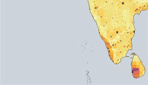
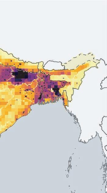
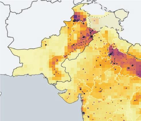
Source: World Bank.
Note: HAP = household air pollution.
These benefits vary by location, according to the geographical distribution of exposure to air pollution. The spatial pattern of ambient air pollution deaths (map 4.2) reflects population density and ambient concentrations. The modeling suggests that deaths will be highest on India’s Indo-Gangetic Plain, in Bangladesh, and in the Punjab area of Pakistan. The Indo-Gangetic Plain, which will contain 40 percent of India’s population in 2030, will account for 47 percent of ambient air pollution deaths. The western states of Gujarat, Maharashtra, and Rajasthan, with 21 percent of India’s 2030 population, will account for 22 percent; and states in the south of India—Andhra Pradesh, Karnataka, Kerala, Tamil Nadu, and Telangana—which together will make up 22 percent of the country’s 2030 population, will account for 18 percent of ambient air pollution deaths.
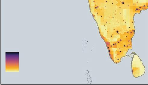
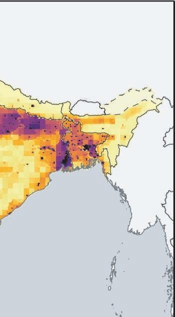
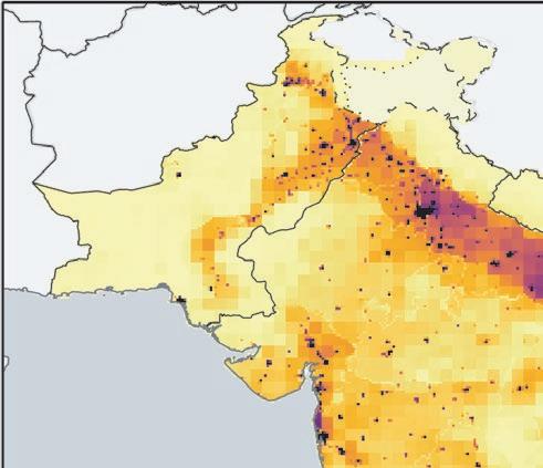
Deaths due to HAP mirror the geographical pattern of HAP exposure (map 4.1). Within India, 45 percent of deaths from HAP are predicted to occur on the Indo-Gangetic Plain; the states in central and eastern India— Chhattisgarh, Madhya Pradesh, and Odisha—account for 17 percent of HAP deaths; while Gujarat, Maharashtra, and Rajasthan account for 16 percent; and Andhra Pradesh, Karnataka, Kerala, Tamil Nadu, and Telangana, in the south of the country, account for 13 percent. Although the absolute number of deaths attributable to HAP will be smaller in 2030 in Nepal, at

25,100 deaths, and Sri Lanka, at 12,600, than in India and Pakistan (table 4.3), 68 percent of PM2.5 deaths in Nepal and Sri Lanka will be attributable to HAP.
Let M represent total observed deaths (for some cause of death) in a grid square. Then

where λT denotes the death rate at the background level of particulate matter (PM) in each grid square, RR(z) is the relative risk of death at exposure level z, pop is the population of the grid square, and pH is the fraction of population in the grid square exposed to both ambient air pollution (AAP) and HAP. Baseline deaths for each subgroup are given by
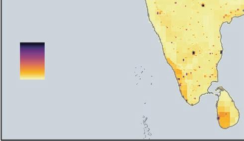
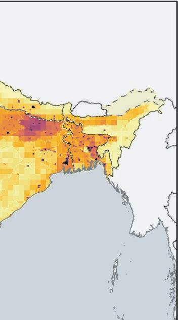
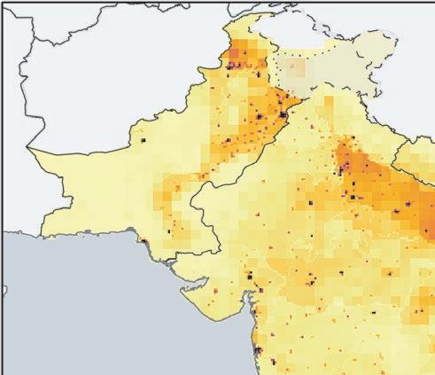
and the result substituted into equations (4.6) and (4.7) to solve for Baseline deathsAAP+HAP and Baseline deathsAAP.
To compute the deaths attributable to ambient and household PM2.5, deaths for each 0.1 × 0.1–degree grid square are calculated by cause of death, and then summed across all causes of death. First, the calculations of ambient PM2.5 (AAP) deaths (applied to each cause of death) are calculated allowing for exposure to HAP, followed by deaths attributable to HAP.
Ambient PM2.5 (PM A) affects both households that use solid fuel for cooking and those that do not. Let pH represent the fraction of the population in a grid square that is exposed to solid fuel from cooking and PMH represent their additional PM2.5 exposure over and above PMA. Then 1−pH of the population is exposed only to PMA. The total deaths due to PM2.5 in the grid square (computed for each cause of death) is given by
where Baseline deathsAAP+HAP represents the total deaths among people exposed to both AAP and HAP and Baseline deathsAAP represents total deaths among those exposed only to AAP (see below for calculation of Baseline deathsAAP and Baseline deathsAAP+HAP). Let RR(z) represent the relative risk of death at PM = z. The population-attributable fraction (PAF) is the proportion of deaths attributable to PM and is given by
The PAF is evaluated at z = PMA+PMH for persons exposed to both AAP and HAP and evaluated at z = PMA for persons exposed only to AAP.6 Baseline deaths for each subgroup in the population can be calculated from total deaths (M), pH, and the relative risk function, as described below. The total deaths attributable to AAP are calculated as
which assumes that AAP deaths among people exposed to both sources of particulate matter are proportional to the share of PMA in total PM2.5 exposure.
When deaths are calculated ignoring HAP, the term in equation (4.4) disappears, and Baseline deathsAAP are equal to total deaths (for each cause) in the grid square (M). Deaths attributable to HAP are given by
When air pollution control strategies reduce ambient PM2.5, the improvement in PMA constitutes a marginal reduction in PM2.5. The deaths avoidable by reducing PMA from PMA0 to PMA1 are measured by the reduction in the risk of death from moving from PMA0 to PMA1 multiplied by baseline deaths.
This formula assumes that neither PMH nor pH is affected by the policy. When either PMH or pH is altered, the change in deaths due to the policy is given by
The relative risk of death is computed as a function of total PM2.5 exposure for each of the six causes of death: ischemic heart disease, strokes, chronic obstructive lung disease, lower respiratory infections, type 2 diabetes, and lung cancer. Exposure-response functions come from the 2019 Global Burden of Disease Study (Global Burden of Disease Collaborative Network 2020). Figure 4A.1 illustrates the exposure-response function for ischemic heart disease for people age 65–70 years.
To compute baseline deaths by disease in 2030 (M), estimates of population for each grid square from the International Institute for Applied Systems Analysis (IIASA) were used, along with death rates by disease from the Institute for Health Metrics and Evaluation (IHME 2021). The proportion of the population in each region exposed to solid fuel (pH) is estimated by the IIASA. PM2.5 exposure associated with HAP, conditional on being exposed, is given by region in table 4A.1.
Source: Original figure for this publication.
Note: PM2.5 (μg/m 3 ) = fine particulate matter measured in micrograms per cubic meter.
(table continued next page)
There is now growing evidence of increased rates of COVID-19 (coronavirus) infection in areas with high levels of air pollution. Air pollution causes cellular damage and inflammation throughout the body and has been linked to higher rates of diseases, including cancer, heart disease, strokes, diabetes, asthma, and other co-morbidities. All these conditions also potentially increase the risk of death for COVID-19 patients.
A study in the United States by Wu et al. (2020) finds that someone living in an area of high particulate pollution is 8 percent more likely to die from COVID-19 than others living in an area with just one unit (μg/m3) less pollution. This study and other similar studies conducted elsewhere and summarized below conclude that a small increase in long-term exposure to pollution can cause larger increases in the COVID-19 death rate. Given that the South Asia region is one of the major global hotspots for air pollution, one could therefore expect increased COVID-19-related cases and deaths linked to air pollution exposure.
In another study, Fattorini and Regoli (2020) attempt to provide evidence on the possible influence of air quality, particularly in terms of chronicity of exposure, on the spread of COVID-19 in Italian regions. They show that long-term air quality data are significantly correlated with cases of COVID-19 in up to 71 Italian provinces, providing evidence that chronic exposure to atmospheric contamination may be an important factor in the spread of the COVID-19 virus. They conclude that atmospheric and environmental pollution should be considered part of an integrated approach to human health protection and the prevention of epidemics from a longterm and chronic perspective.
Zhu et al. (2020) explore the relationship between ambient air pollutants and the infection caused by the COVID-19 virus in China, which experienced the first set of cases in the world. They use data from daily confirmed cases, air pollution concentration, and meteorological variables in 120 cities to investigate the associations of six air pollutants (fine particulate matter [PM2.5], particulate matter [PM10], sulfur dioxide [SO₂], carbon monoxide [CO], nitrogen oxides [NO₂], and ozone [O₃]) with confirmed COVID-19 cases. Their findings suggest that a 10 μg/m3 increase in PM2.5, PM10, NO₂, and O₃ was associated with a 2.24, 1.76, 6.94, and 4.76 percent increase in the daily counts of confirmed cases, respectively, at a 95 percent confidence interval.
Using spatial econometric technics, Cole, Ozgen, and Strobl (2020) examine the correlation between long-term air pollution exposure and COVID-19 using data for 355 relatively small Dutch municipalities. They estimate long-term exposure to concentrations of PM2.5, NO₂, and SO₂ on the number of COVID-19 infections; individuals hospitalized with COVID-19; and those who died because of COVID-19. Their results indicate that a 1 μ/m3 increase in PM2.5 concentration is associated with 9.4 more COVID-19 cases, 3.0 more hospital admissions, and 2.3 more deaths.
Yamada, Yamada, and Mani (2020) examine the case of India, one of the countries with the highest levels of ambient air pollution and HAP, and investigate links to the COVID-19 fatality rate using district-level data. The results suggest a positive and statistically significant association between exposure to HAP and COVID-19 fatality rates. The estimation results indicate that a 1 percent increase in long-term exposure to PM2.5 is associated with an increase in COVID-19 deaths of 5.7 percentage points and an increase in the COVID-19 fatality rate of 0.027 percentage point, but this exposure is not necessarily correlated with COVID-19 cases. People with underlying health conditions such as respiratory illness caused by exposure to air pollution might have a higher risk of death following SARS-CoV-2 infection. This finding might also apply to other developing countries where high levels of air pollution are a critical issue for development and public health.
1. UNICEF, “Stop Stunting in Asia, Part 1,” https://www.unicef.org/rosa/stories/stop-stunting-south -asia-part-1.
2. Table 4A.1 presents estimates of deaths due to ambient and household air pollution for each of the 31 regions in the study area.
3. Deaths due to each of these causes in 2030 are projected using the population estimates in this study and death rate projections from the Institute for Health Metrics and Evaluation (table 4A.2 in annex 4A).
4. The attributable fraction is multiplied by the baseline number of deaths for each group, by disease, to estimate the total deaths attributable to air pollution (annex 4A). For people exposed only to ambient air pollution, deaths attributed to PM2.5 are labeled as deaths attributable to ambient PM2.5 For those exposed to both ambient and household air pollution, deaths attributable to ambient PM2.5 equal total deaths attributable to PM2.5 multiplied by the fraction of total exposure due to ambient air pollution.
5. If exposure-response functions were not concave, the fraction of deaths attributable to air pollution would be astronomical. The concavity of exposure-response functions is caused by several factors. Data on active smokers show that there are limits to health effects from very high doses of particulate matter. Concavity also reflects the fact that sensitive people die at lower doses of particulate matter. Those who survive are more resilient.
6. For a person for whom household air pollution is > 0, what is added to ambient PM2.5 is a measure of total indoor exposure, which depends on type of fuel burned and amount of time spent indoors, minus ambient PM2.5 exposure. Thus, “additional PM2.5 exposure due to household air pollution” is added to ambient PM2.5 to measure exposure for someone exposed to both ambient and household air pollution.
Aguilar-Gomez, Sandra, Holt Dwyer, Joshua S. Graff Zivin, and Matthew J. Neidell. 2022. “This Is Air: The ‘Non-Health’ Effects of Air Pollution.” Annual Review of Resource Economics 14 (1): 403–25.
Alberini, Anna, Maureen Cropper, Alan Krupnick, and Nathalie B. Simon. 2004. “Does the Value of a Statistical Life Vary with Age and Health Status? Evidence from the US and Canada.” Journal of Environmental Economics and Management 48 (1): 769–92.
Al-Kindi, Sadeer G., Robert D. Brook, Shyam Biswal, and Sanjay Rajagopalan. 2020. “Environmental Determinants of Cardiovascular Disease: Lessons Learned from Air Pollution.” Nature Reviews Cardiology 17 (10): 656–72.
Almond, Douglas, and Janet Currie. 2011. “Killing Me Softly: The Fetal Origins Hypothesis.” Journal of Economic Perspectives 25 (3): 153–72.
Anderson, Michael L. 2020. “As the Wind Blows: The Effects of Long-Term Exposure to Air Pollution on Mortality.” Journal of the European Economic Association 18 (4): 1886–927.
Apte, Joshua S., Michael Brauer, Aaron J. Cohen, Majid Ezzati, and C. Arden Pope III. 2018. “Ambient PM2.5 Reduces Global and Regional Life Expectancy.” Environmental Science and Technology Letters 5 (9): 546–51.
Arceo, Eva, Rema Hanna, and Paulina Oliva. 2016. “Does the Effect of Pollution on Infant Mortality Differ between Developing and Developed Countries? Evidence from Mexico City.” Economic Journal 126 (591): 257–80.
Balakrishnan, Kalpana, Sagnik Dey, Tarun Gupta, R. S. Dhaliwal, Michael Brauer, Aaron J. Cohen, Jeffrey D. Stanaway, et al. 2019. “The Impact of Air Pollution on Deaths, Disease Burden, and Life Expectancy across the States of India: The Global Burden of Disease Study 2017.” The Lancet Planetary Health 3 (1): e26–39.
Balakrishnan, Uttara, and Magda Tsaneva. 2021. “Air Pollution and Academic Performance: Evidence from India.” World Development 146: 105553.
Barker, David J. 1995. “Fetal Origins of Coronary Heart Disease.” British Medical Journal 311 (6998): 171.
Bharadwaj, Prashant, and Juan Eberhard. 2008. “Atmospheric Air Pollution and Birth Weight.” Unpublished, Department of Economics, Yale University, New Haven, CT.
Bharadwaj, Prashant, Matthew Gibson, Joshua Graff Zivin, and Christopher Neilson. 2017. “Gray Matters: Fetal Pollution Exposure and Human Capital Formation .” Journal of the Association of Environmental and Resource Economists 4 (2): 505–42.
Bishop, Kelly C., Jonathan D. Ketcham, and Nicolai V. Kuminoff. 2018. “Hazed and Confused: The Effect of Air Pollution on Dementia.” Working Paper 24970, National Bureau of Economic Research, Cambridge, MA.
Bobak, Martin, Marcus Richards, and Michael Wadsworth. 2004. “Relation between Children’s Height and Outdoor Air Pollution from Coal-Burning Sources in the British 1946 Birth Cohort.” International Archives of Occupational and Environmental Health 77 (6): 383–86.
Bozzoli, Carlos, Angus Deaton, and Climent Quintana-Domeque. 2009. “Adult Height and Childhood Disease.” Demography 46 (4): 647–69.
Brockmeyer, Sam, and Amedeo D’Angiulli. 2016. “How Air Pollution Alters Brain Development: The Role of Neuroinflammation.” Translational Neuroscience 7 (1): 24–30. https:// doi.org/10.1515/tnsci -2016-0005.
Burnett, Richard T., C. Arden Pope III, Majid Ezzati, Casey Olives, Stephen S. Lim, Sumi Mehta, Hwashin H. Shin, et al. 2014. “An Integrated Risk Function for Estimating the Global Burden of Disease Attributable to Ambient Fine Particulate Matter Exposure.” Environmental Health Perspectives 122 (4): 397– 403.
Calderón-Garcidueñas, Lilian, Amedeo D’Angiulli, Randy J. Kulesza, Ricardo Torres-Jardón, Norma Osnaya, Lina Romero, Sheyla Keefe, et al. 2011. “Air Pollution Is Associated with Brainstem Auditory Nuclei Pathology and Delayed Brainstem Auditory Evoked Potentials.” International Journal of Developmental Neuroscience 29 (4): 365–75.
Chang, Tom Y., Joshua Graff Zivin, Tal Gross, and Matthew Neidell. 2019. “The Effect of Pollution on Worker Productivity: Evidence from Call Center Workers in China.” American Economic Journal: Applied Economics 11 (1): 151–72.
Chen, Hong, Jeffrey C. Kwong, Ray Copes, Perry Hystad, Aaron van Donkelaar, Karen Tu, Jeffrey R. Brook, et al. 2017. “Exposure to Ambient Air Pollution and the Incidence of Dementia: A PopulationBased Cohort Study.” Environment International 108: 271–77.
Chen, Shuai, Paulina Oliva, and Peng Zhang. 2018. “Air Pollution and Mental Health: Evidence from China.” Working Paper 24686, National Bureau of Economic Research, Cambridge, MA.
Chen, Yuyu, Avraham Ebenstein, Michael Greenstone, and Hongbin Li. 2013. “Evidence on the Impact of Sustained Exposure to Air Pollution on Life Expectancy from China’s Huai River Policy.” Proceedings of the National Academy of Sciences 110 (32): 12936–41.
Chowdhury, Sourangsu, Sagnik Dey, Sarath Guttikunda, Ajay Pillarisetti, Kirk R. Smith, and Larry Di Girolamo. 2019. “Indian Annual Ambient Air Quality Standard Is Achievable by Completely Mitigating Emissions from Household Sources.” Proceedings of the National Academy of Sciences 116 (22): 10711–16.
Cohen, Aaron J., H. Ross Anderson, Bart Ostro, K. Dev Pandey, Michal Krzyzanowski, Nino Künzli, Kersten Gutschmidt, et al. 2004. “Urban Air Pollution.” In Comparative Quantification of Health Risks: Global and Regional Burden of Disease Attributable to Selected Major Risk Factors, Volume 2, edited by Majid Ezzati, Alan D. Lopez, Anthony Rodgers, and Christopher J. L. Murray,1353–433. Geneva: World Health Organization.
Cohen, Aaron J., Michael Brauer, Richard Burnett, H. Ross Anderson, Joseph Frostad, Kara Estep, Kalpana Balakrishnan, et al. 2017. “Estimates and 25-Year Trends of the Global Burden of Disease Attributable to Ambient Air Pollution: An Analysis of Data from the Global Burden of Diseases Study 2015.” The Lancet 389 (10082): 1907–18.
Cole, Matthew A., Ceren Ozgen, and Eric Strobl. 2020. “Air Pollution Exposure and COVID-19.” IZA Discussion Paper 13367, Institute of Labor Economics, Bonn.
Cropper, Maureen, James K. Hammitt, and Lisa A. Robinson. 2011. “Valuing Mortality Risk Reductions: Progress and Challenges.” Annual Review of Resource Economics 3 (1): 313–36.
Currie, Janet, and Douglas Almond. 2011. “Human Capital Development before Age Five.” Handbook of Labor Economics 4: 1315–486.
Currie, Janet, Joshua Graff Zivin, Jamie Mullins, and Matthew Neidell. 2014. “What Do We Know about Short-and Long-Term Effects of Early-Life Exposure to Pollution?” Annual Review of Resource Economics 6 (1): 217–47.
Currie, Janet, and Tom Vogl. 2013. “Early-Life Health and Adult Circumstance in Developing Countries.” Annual Review of Economics 5: 1–36.
Deschenes, Olivier, Huixia Wang, Si Wang, and Peng Zhang. 2020. “The Effect of Air Pollution on Body Weight and Obesity: Evidence from China.” Journal of Development Economics 145: 102461.
Ebenstein, Avraham, Maoyong Fan, Michael Greenstone, Guojun He, Peng Yin, and Maigeng Zhou. 2015. “Growth, Pollution, and Life Expectancy: China from 1991–2012.” American Economic Review 105 (5): 226–31.
Ebenstein, Avraham, Maoyong Fan, Michael Greenstone, Guojun He, and Maigeng Zhou. 2017. “New Evidence on the Impact of Sustained Exposure to Air Pollution on Life Expectancy from China’s Huai River Policy.” Proceedings of the National Academy of Sciences 114 (39): 10384–89.
Fattorini, Daniele, and Francesco Regoli. 2020. “Role of the Chronic Air Pollution Levels in the COVID-19 Outbreak Risk in Italy.” Environmental Pollution 264: 114732. https:// doi. org/10.1016/j. envpol.2020.114732.
Frankenberg, Elizabeth, Douglas McKee, and Duncan Thomas. 2005. “Health Consequences of Forest Fires in Indonesia.” Demography 42 (1): 109–29.
Galasso, Emanuela, and Adam Wagstaff. 2019. “The Aggregate Income Losses from Childhood Stunting and the Returns to a Nutrition Intervention Aimed at Reducing Stunting.” Economics and Human Biology 34 (2019): 225–38.
Global Burden of Disease Collaborative Network. 2020. “Global Burden of Disease Study 2019 (GBD 2019) Relative Risks.” Institute for Health Metrics and Evaluation (IHME), Seattle.
Goyal, Nihit, and David Canning. 2018. “Exposure to Ambient Fine Particulate Air Pollution in Utero as a Risk Factor for Child Stunting in Bangladesh.” International Journal of Environmental Research and Public Health 15 (1): 22.
Goyal, Nihit, Mahesh Karra, and David Canning. 2019. “Early-Life Exposure to Ambient Fine Particulate Air Pollution and Infant Mortality: Pooled Evidence from 43 Low-and Middle-Income Countries.”
International Journal of Epidemiology 48 (4): 1125–41.
Graff Zivin, Joshua, and Matthew Neidell. 2012. “The Impact of Pollution on Worker Productivity.”
American Economic Review 102 (7): 3652–73.
Greenstone, Michael, and Rema Hanna. 2014. “Environmental Regulations, Air and Water Pollution, and Infant Mortality in India.” American Economic Review 104 (10): 3038–72.
Greenstone, Michael, Janhavi Nilekani, Rohini Pande, Nicholas Ryan, Anant Sudarshan, and Anish Sugathan. 2015. “Lower Pollution, Longer Lives: Life Expectancy Gains If India Reduced Particulate Matter Pollution.” Economic and Political Weekly 50 (8): 40–46.
Gupta, Usha. 2008. “Valuation of Urban Air Pollution: A Case Study of Kanpur City in India.” Environmental and Resource Economics 41 (3): 315–26.
Hanna, Rema, Esther Duflo, and Michael Greenstone. 2016. “Up in Smoke: The Influence of Household Behavior on the Long-Run Impact of Improved Cooking Stoves.” American Economic Journal: Economic Policy 8 (1): 80–114.
Hanna, Rema, and Paulina Oliva. 2016. “Implications of Climate Change for Children in Developing Countries.” The Future of Children 26 (1): 115–32.
He, Jiaxiu, Haoming Liu, and Alberto Salvo. 2019. “Severe Air Pollution and Labor Productivity: Evidence from Industrial Towns in China.” American Economic Journal: Applied Economics 11 (1): 173–201. Health Effects Institute. 2011. “Public Health and Air Pollution in Asia (PAPA): Coordinated Studies of Short-Term Exposure to Air Pollution and Daily Mortality in Two Indian Cities.” Research Report 157, Health Effects Institute, Boston.
Heft-Neal, Sam, Martin Heger, Vaibhav Rathi, and Marshall Burke. 2022. “Identifying Child Growth Effects of Elevated Pollution Levels during Pregnancy.” Unpublished, Working Paper, World Bank, Washington, DC.
Heger, Martin, Gregor Zens, and Craig Meisner. 2019. “Particulate Matter, Ambient Air Pollution, and Respiratory Disease in Egypt.” World Bank, Washington, DC.
IHME (Institute for Health Metrics and Evaluation). 2021. “Global Health Data Exchange | GHDx.” IHME, Seattle.
Janke, Katharina. 2014. “Air Pollution, Avoidance Behaviour and Children’s Respiratory Health: Evidence from England.” Journal of Health Economics 38: 23–42.
Jayachandran, Seema. 2009. “Air Quality and Early-Life Mortality: Evidence from Indonesia’s Wildfires.” Journal of Human Resources 44 (4): 916–54.
Kahn, Matthew E., and Pei Li. 2019. “The Effect of Pollution and Heat on High-Skill Public Sector Worker Productivity in China.” Working Paper 25594, National Bureau of Economic Research, Cambridge, MA.
Kajekar, Radhika. 2007. “Environmental Factors and Developmental Outcomes in the Lung.” Pharmacology and Therapeutics 114 (2): 129–45.
Kar, Abhishek, Shonali Pachauri, Rob Bailis, and Hisham Zerriffi. 2019. “Using Sales Data to Assess Cooking Gas Adoption and the Impact of India’s Ujjwala Programme in Rural Karnataka.” Nature Energy 4 (9): 806–14.
Katsouyanni, K., and APHEA Group. 2006. “APHEA Project: Air Pollution and Health: A European Approach.” Epidemiology 17 (6): S19.
Krishna, Bhargav, Kalpana Balakrishnan, Amna R. Siddiqui, Bilkis A. Begum, Damodar Bachani, and Michael Brauer. 2017. “Tackling the Health Burden of Air Pollution in South Asia.” BMJ 359: j5209.
Krishna, Bhargav, Siddhartha Mandal, Kishore Madhipatla, K. Srinath Reddy, Dorairaj Prabhakaran, and Joel D. Schwartz. 2021. “Daily Nonaccidental Mortality Associated with Short-Term PM2.5 Exposures in Delhi, India.” Environmental Epidemiology 5 (44): e167.
Landrigan, Philip J., Richard Fuller, Nereus J .R. Acosta, Olusoji Adeyi, Robert Arnold, Abdoulaye Bibi Baldé, Roberto Bertollini, et al. 2018. “The Lancet Commission on Pollution and Health.” The Lancet 391 (10119): 462–512.
Lelieveld, Jos, Andy Haines, and Andrea Pozzer. 2018. “Age-Dependent Health Risk from Ambient Air Pollution: A Modelling and Data Analysis of Childhood Mortality in Middle-Income and Low-Income Countries.” The Lancet Planetary Health 2 (7): e292–300.
Lelieveld, Jos, Andrea Pozzer, Ulrich Pöschl, Mohammed Fnais, Andy Haines, and Thomas Münzel. 2020. “Loss of Life Expectancy from Air Pollution Compared to Other Risk Factors: A Worldwide Perspective.” Cardiovascular Research 116 (11): 1910–17.
Li, Shi, Stuart Batterman, Elizabeth Wasilevich, Robert Wahl, Julie Wirth, Feng-Chiao Su, and Bhramar Mukherjee. 2011. “Association of Daily Asthma Emergency Department Visits and Hospital Admissions with Ambient Air Pollutants among the Pediatric Medicaid Population in Detroit: Time-Series and Time-Stratified Case-Crossover Analyses with Threshold Effects.” Environmental Research 111 (8): 1137–47.
Lim, Stephen S., Theo Vos, Abraham D. Flaxman, Goodarz Danaei, Kenji Shibuya, Heather Adair-Rohani, Mohammad A. AlMazroa, et al. 2012. “A Comparative Risk Assessment of Burden of Disease and Injury Attributable to 67 Risk Factors and Risk Factor Clusters in 21 Regions, 1990–2010: A Systematic Analysis for the Global Burden of Disease Study 2010.” The Lancet 380 (9859): 2224–60.
Liu, Ya-Ming, and Chon-Kit Ao. 2021. “Effect of Air Pollution on Health Care Expenditure: Evidence from Respiratory Diseases.” Health Economics 30 (4): 858–75.
Mani, Muthukumara, and Takahiro Yamada. 2020. “Is Air Pollution Aggravating COVID-19 in South Asia?” World Bank Blogs, June 23.
Misra, Anoop, Nikhil Tandon, Shah Ebrahim, Naveed Sattar, Dewan Alam, Usha Shrivastava, KM Venkat Narayan, and Tazeen H. Jafar. 2017. “Diabetes, Cardiovascular Disease, and Chronic Kidney Disease in South Asia: Current Status and Future Directions.” BMJ 357: j1420.
Moretti, Enrico, and Matthew Neidell. 2011. “Pollution, Health, and Avoidance Behavior: Evidence from the Ports of Los Angeles.” Journal of Human Resources 46 (1): 154–75.
Murray, Christopher J. L., Aleksandr Y. Aravkin, Peng Zheng, Cristiana Abbafati, Kaja M. Abbas, Mohsen Abbasi-Kangevari, Foad Abd-Allah, et al. 2020. “Global Burden of 87 Risk Factors in 204 Countries and Territories, 1990–2019: A Systematic Analysis for the Global Burden of Disease Study 2019.” The Lancet 396 (10258): 1223–49.
Narain, Urvashi, and Chris Sall. 2016. “Methodology for Valuing the Health Impacts of Air Pollution.” World Bank, Washington, DC. https://doi.org/10.1596/24440.
Pedersen, Marie, Lise Giorgis-Allemand, Claire Bernard, Inmaculada Aguilera, Anne-Marie Nybo Andersen, Ferran Ballester, Rob M. J. Beelen, et al. 2013. “Ambient Air Pollution and Low Birthweight: A European Cohort Study (ESCAPE).” The Lancet Respiratory Medicine 1 (9): 695–704.
Peters, Annette, and C. Arden Pope III. 2002. “Cardiopulmonary Mortality and Air Pollution.” The Lancet 360 (9341): 1184–85.
Pope, C. Arden III, Richard T. Burnett, Michael J. Thun, Eugenia E. Calle, Daniel Krewski, Kazuhiko Ito, and George D. Thurston. 2002. “Lung Cancer, Cardiopulmonary Mortality, and Long-Term Exposure to Fine Particulate Air Pollution.” JAMA 287 (9): 1132–41.
Rehfuess, E., D. Pope, N. Bruce, M. Dherani, K. Jagoe, L. Naeher, and C. Noonan. 2014. “Review 6: Impacts of Interventions on Household Air Pollution Concentrations and Personal Exposure.” WHO Indoor Air Quality Guidelines: Household Fuel Combustion . Geneva: World Health Organization.
Robinson, Lisa A., James K. Hammitt, and Lucy O’Keeffe. 2019. “Valuing Mortality Risk Reductions in Global Benefit-Cost Analysis.” Journal of Benefit-Cost Analysis 10 (S1): 15–50. https://doi.org/10.1017 /bca.2018.26.
Rosales-Rueda, Maria, and Margaret Triyana. 2019. “The Persistent Effects of Early-Life Exposure to Air Pollution: Evidence from the Indonesian Forest Fires.” Journal of Human Resources 54 (4): 1037–80.
Samet, Jonathan M., Francesca Dominici, Frank C. Curriero, Ivan Coursac, and Scott L. Zeger. 2000. “Fine Particulate Air Pollution and Mortality in 20 US Cities, 1987–1994.” New England Journal of Medicine 343 (24): 1742–49.
Singh, Nandita, Vishnu Murari, Manish Kumar, S. C. Barman, and Tirthankar Banerjee. 2017. “Fine Particulates over South Asia: Review and Meta-Analysis of PM2.5 Source Apportionment through Receptor Model.” Environmental Pollution 223: 121–36.
Sinharoy, Sheela S., Thomas Clasen, and Reynaldo Martorell. 2020. “Air Pollution and Stunting: A Missing Link?” The Lancet Global Health 8 (4): e472–75.
Smith, Kirk R., and Ajay Pillarisetti. 2017. “Household Air Pollution from Solid Cookfuels and Its Effects on Health.” In Injury Prevention and Environmental Health, third edition, Disease Control Priorities, Volume 7, edited by Charles N. Mock, Rachel Nugent, Olive Kobusingye, and Kirk R. Smith. Washington, DC: World Bank.
Suades-González, Elisabet, Mireia Gascon, Mònica Guxens, and Jordi Sunyer. 2015. “Air Pollution and Neuropsychological Development: A Review of the Latest Evidence.” Endocrinology 156 (10): 3473–82.
Viscusi, W. Kip, and Joseph E. Aldy. 2003. “The Value of a Statistical Life: A Critical Review of Market Estimates throughout the World.” Journal of Risk and Uncertainty 27 (1) 1: 5–76.
WHO (World Health Organization). 2021. “Ambient (Outdoor) Air Pollution.” Geneva, WHO.
Wong, Chit-Ming, Nuntavarn Vichit-Vadakan, Haidong Kan, and Zhengmin Qian. 2008. “Public Health and Air Pollution in Asia (PAPA): A Multicity Study of Short-Term Effects of Air Pollution on Mortality.” Environmental Health Perspectives 116 (9): 1195–202.
World Bank. 2022. The Global Health Cost of PM2.5 Air Pollution: A Case for Action beyond 2021 International Development in Focus. Washington, DC: World Bank.
Wu, X., R. C. Nethery, M. B. Sabath, D. Braun, and F. Dominici. 2020. “Air Pollution and COVID-19 Mortality in the United States: Strengths and Limitations of an Ecological Regression Analysis.” Science Advance 6 (45): eabd4049. doi:10.1126/sciadv.abd4049.
Yamada, Takahiro, Hiroyuki Yamada, and Muthukumara Mani. 2020. “The Causal Effects of Long-Term PM2.5 Exposure on COVID-19 in India.” Policy Research Working Paper 9543, World Bank, Washington, DC.
Zhao, Bin, Shuxiao Wang, Dian Ding, Wenjing Wu, Xing Chang, Jiandong Wang, Jia Xing, Carey Jang, Joshua S. Fu, and Yun Zhu. 2019. “Nonlinear Relationships between Air Pollutant Emissions and PM2.5-Related Health Impacts in the Beijing-Tianjin-Hebei Region.” Science of the Total Environment 661: 375–85.
Zhu, Yongjian, Jingui Xie, Fengming Huang, and Liqing Cao. 2020. “Association between Short-Term Exposure to Air Pollution and COVID-19 Infection: Evidence from China.” Science of the Total Environment 727 (20): 138704.
Governments in South Asia are increasingly putting policies in place to reduce air pollution. The draft Bangladesh Clean Air Act, India’s National Clean Air Programme, and the National Electric Vehicles Policy in Pakistan are examples of these policies, which mainly focus on power generation, transportation, and large industries. Bangladesh, India, Nepal, Pakistan, and Sri Lanka have all imposed varying emissions standards for vehicles, and mandate low–nitrogen oxide (low-NOx) burners for power plants and filters for some large industrial boilers. These policies can prevent further worsening of air quality even with substantial economic growth going forward. However, much more is needed to significantly reduce the current dangerous levels of air pollution.
In India, first steps are being taken to introduce cleaner cooking fuel for households, more efficient brick kilns, and better solid waste management. However, even after full implementation of current policies, 30 percent of households in India will still be using biomass for cooking, and the transformation will be incomplete in the other two areas. That also means that in India, significant progress at relatively low cost is still possible in these areas. In addition, abatement efforts (government investments and monitoring) in India, as well as in other countries in South Asia, are still predominantly focused on large cities.
A major limitation of the current policies is that they focus on emissions and air quality within cities. Such an approach is insufficient because, in most South Asian cities, more than half the air pollution originates from outside those cities; meanwhile, the polluting emissions inside cities worsen air quality far beyond city borders. In other words, air pollution in cities is part of the pollution of much larger airsheds caused by emissions from a wide range of sources. The problem of a city-focused approach is twofold. First, it is extremely expensive, if not impossible, to significantly improve air quality in cities with only in-city abatement policies, given that these policies need to compensate for pollution that comes from outside the city, and abatement costs in industry and transportation are significantly higher than abatement in agriculture. Second, public support for such policies is limited because their impact on the city itself is limited. Cities are strongly tempted to blame neighboring areas rather than taking action themselves.
The limitations of a city-focused approach mean that cooperation between different jurisdictions within an airshed becomes crucial. If every single area can rely on the commitment of other areas in the same airshed, lower-cost abatement is sufficient to reach goals everywhere and support for abatement policies increases. This concept is illustrated in figure 5.1 for the most cost-effective scenario discussed in chapter 3. Even with maximum, and thus expensive, local efforts within the states and provinces of the Indo-Gangetic Plain (IGP), the local air quality target (World Health Organization [WHO] Interim Target 1) cannot be reached if areas outside the state or province do not also reduce emissions, whereas the target is easily within reach with combined efforts of all surrounding states and provinces. Such cooperation across different areas has the additional advantage of leveling the playing field for pollution producers in these areas: they all face the same restrictions on polluting forms of production. Once such a level of coordination is in place, it becomes possible to achieve leastcost improvement in air quality by reducing emissions more in places where abatement costs are initially lower. Such solutions require economic incentives so that the burden of the abatement costs is shared by everybody who benefits from the emissions reductions. This sharing can be accomplished by establishing regional funds or even by introducing a system of tradable emissions rights.
Airsheds do not recognize national borders. Based on the analysis in chapter 2, map 5.1 provides two examples of airsheds in the IGP, including states and provinces, or other jurisdictions of India, Nepal, and Pakistan. The airshed in panel a covers the western and central parts of the IGP, and the airshed in panel b covers the eastern part of the IGP. Given the predominant wind direction from the northwest to the southeast, 30 percent of the air pollution in the Indian state of Punjab comes from Punjab Province in Pakistan and, on average, 30 percent of the air pollution in the largest cities of Bangladesh (Chittagong, Dhaka, and Khulna) originates in India. However, during some months of the year, substantial pollution flows in the opposite direction across borders.
Possible improvements if all available local measures were taken
Improvement from measures taken in other regions
Possible improvements if all available measures in other regions were taken
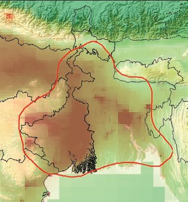
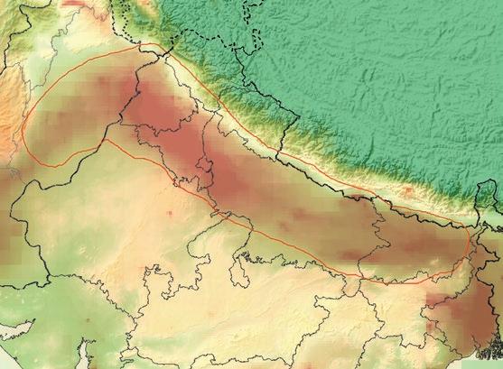
a. Suggested airshed covering the western and central par ts of the IGPb. Suggested airshed covering the eastern par t of the IGP
Source: Original map for this publication.
Note: Colors indicate fine particulate matter concentrations in 2018, measured in micrograms per cubic meter. IGP = Indo-Gangetic Plain.
Establishing effective coordination is challenging, but several successful mechanisms have been developed around the world. In China, Europe, and the United States, air quality policies have transformed attitudes of blaming the neighbors and free-riding behaviors into constructive cooperation that delivers important public health and economic benefits. Common elements of these coordination efforts include (1) an overarching regulatory framework that sets emissions and air quality targets for participating jurisdictions, (2) a well-funded central institution that ensures accountability and transparency, (3) decentralized planning of abatement policies within the parameters set centrally, and (4) economic incentives to reduce emissions, for example, through taxes and subsidies or by making access to funds conditional on abatement performance (see box 5.1).
Building on the analysis in this report and on successful policy coordination around the world, a schematic road map for airshedwide air quality management (AQM) can be drawn. Such a road map consists of three phases, with each phase broken down into three distinct steps (table 5.1). The first phase sets the condition for airshedwide coordination and cooperation. During this phase, the monitoring of air pollution is expanded beyond the big cities, data are shared with the public, credible scientific institutes that analyze the airshed are created or strengthened, and the national government moves to a whole-of-government approach. In the second phase, abatement interventions are broadened beyond the traditional targets of power plants, large factories, and transportation. During this phase, major progress can be made in reducing air pollution from agriculture, solid waste management, cookstoves, brick kilns, and other small industries. At the same time, airshedwide standards are introduced. In the third phase, AQM is mainstreamed into economic policy. During this phase, economic incentives are fine-tuned to allow private sector solutions, to the maximum extent possible, to address distributional impacts and to exploit synergies with climate change policies. In this phase, trading of emissions permits can also be introduced to optimize abatement across jurisdictions and across firms.

California. The state of California was one of the first places in the world to apply an airshed management approach. With a growing understanding that pollution from vehicles, power plants, and industry crossed county jurisdictions, California established 35 air-quality-management districts (AQMD) in the late 1950s that were then further grouped into 15 air basins (airsheds) closely following the topography of the state (map B5.1.1). To coordinate air quality management (AQM) throughout the state, the California Air Resources Board was established with a mandate to manage air pollution sources that have statewide impacts, mostly mobile sources, while each AQMD has the mandate to manage mostly stationary sources that can be controlled within its district. The board also has the responsibility for building up the regulatory, technical, and administrative AQM capacity of the state. The state has committed a large group of staff and substantial financial resources to this activity. Each AQMD is responsible for planning, budgeting, and implementation within its territory. Further management planning and implementation coordination were established within each air basin. Finally, implementation of this model has been incentivized by the federal government: federal funds are withheld if the state fails to attain air quality standards. Based on the AQMD and air basin structure coordinated by the California Air Resources Board, the state has been able to improve from being the worst air quality location in the United States in the 1950s and 1960s to now imposing the strictest air quality standards in the country.
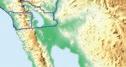


Source: International Institute for Applied Systems Analysis, based on air quality analysis map from US Environmental Protection Agency, available at https://www3.epa.gov/region9/air/maps/ca_clss1.html
Note: Left panel shows 58 counties in California; right panel shows 15 airsheds (air basins).


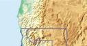


Europe. After recognizing the importance of the long-range transport of air pollution and the resulting need for Europe-wide coordination for AQM policies, the 1979 Convention on Long-Range Transboundary Air Pollution emerged as the first multilateral agreement to address transboundary air pollution in Europe (map B5.1.2). It currently brings together 51 parties, including the former socialist states in Eastern Europe, the Russian Federation, and North America. Informed by a better understanding of air pollution science, the convention has since established systematic monitoring, reporting, and verification mechanisms for ambient air quality, emissions inventories, and policies and measures that are taken by the parties to reduce their emissions. Eight protocols with specific obligations for the signatories to reduce emissions, including implementing quantitative national emissions ceilings that limit the inflow of pollution from other countries, have led to a sharp decoupling of emissions from economic growth.
(box continued next page)


Europe Union ~1,500
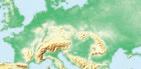
• Air quality limit values (uniform)


• Uniform, source-specific emissions limit values (best available technologies)
• National emissions ceilings


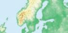
National governments 200–1,000
City administrations 20–50
• Transposition of EU legislation into national laws

• Licensing
• Air quality monitoring
• Air quality management plans


• Local short-term action plans
Acknowledging air pollution as an issue of political concern that requires a coordinated policy response to protect human health and the environment in a cost-effective manner, and to avoid undue distortion of economic competition among its 27 member states, the European Union (EU) has established a more comprehensive framework of air pollution legislation. This legal framework assigns differentiated responsibilities to three administrative levels:
1. EU-wide legislation sets out the air quality objectives, the overall legal framework, and specific EU-wide requirements for ambient air quality, uniform source-specific emissions limit values, and national emissions ceilings that all member states need to meet.
2. Member states must transform all EU-wide legislation into national laws and report on progress, for example, on emissions inventories, monitoring of ambient air quality, policies, and measures.
3. At the subnational level, local authorities and city administrations are responsible for licensing individual plants, conducting air quality monitoring, and developing AQM plans for their regions. If deemed promising, cities might also elaborate on local short-term action plans, although there are doubts about their effectiveness, especially for regional pollutants such as fine particulate matter.
China. Following a high pollution event on the North China Plain in early 2013, the Chinese government established collaboration between the Beijing and Tianjin municipalities, Hebei Province, and parts of the neighboring Henan, Shandong, and Shanxi provinces—the so-called Jing-Jin-Ji area—through which the Beijing Environmental Protection Bureau was assigned to coordinate AQM planning and yearly revisions of the plans of the three jurisdictions (map B5.1.3). The area—which includes the Beijing and Tianjin municipalities and 26 prefectures, all pollution hotspots—has begun applying integrated airshed management. Since 2018, with the establishment of the Department for Regional Air Quality Management, more power was given to the expanded Jing-Jin-Ji coordination body (established in 2013), which coordinates overall AQM planning and implementation. The Chinese Academy of Environmental Sciences supports the coordination body by determining cost-effectiveness and priority measures using a tailored edition of the Greenhouse Gas and Air Pollution Interactions and Synergies (GAINS) program.
(box continued next page)
BOX 5.1 Experiences around the Globe with Coordination to Improve Air Quality (continued )
MAP B5.1.3 The Expanded Jing-Jin-Ji Airshed, with Two Municipalities and 26 Prefectures, on the North China Plain, China
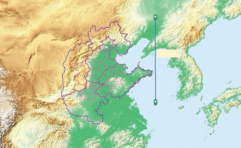
Source: International Institute for Applied Systems Analysis.
Phase
Phase I
Better monitoring and building institutions
Step Action
1 Widespread installment of sensors and sharing of data
2 Creation of credible scientific institutes that analyze airsheds
3 Preparation of a whole-of-government approach Phase
The phases in the road map may overlap when the rate of progress differs, depending on local circumstances. Introducing domestic policies will be easier and will progress faster than establishing cross-border coordination. However, now is the time to initiate cross-border coordination with the steps described in the first phase, even if some of the domestic initiatives have already moved on to a subsequent phase. Cross-border cooperation that lags too far behind would become an insurmountable obstacle to achieving effective and efficient solutions. The phases may also overlap in a different sense: the monitoring and analyses of pollution data will likely evolve throughout the process as economic incentives trigger new technologies and sectoral shifts occur. In addition, the third phase should be kept in mind at the beginning of the process. Even if complete economic solutions are not yet available, it is important to keep the economic incentives in the line of sight from the start. For example, eliminating subsidies for polluting production methods as soon as possible is important. Nevertheless, despite these overlaps, the road map describes logical sequencing. Better data are indispensable for any policy, so data collection and analysis should always come early in the process. Fully fledged economic solutions across borders to allow for the compensation of countries as part of optimal abatement strategies is most challenging.
Cost-effective AQM requires more comprehensive monitoring, enhanced scientific capacity, a shared knowledge base, and strong cooperation between governments. Expanding the number of reliable monitoring devices, including outside cities, is the first step in preparing for airshedwide AQM. A common scientific knowledge base that quantifies key sources of pollution, atmospheric chemistry, and transportation processes; the costs of reducing emissions; and the benefits of clean air for human health and the economy will contribute to a shared understanding of the problems and solutions. Better cooperation between governments is needed to align AQM with climate change policies, distributional policies, and other more general economic policies.
Emissions inventories are currently incomplete in South Asia. South Asia should move toward a comprehensive, unified inventory for the region that represents the full range of relevant emissions sources instead of relying on each city or state to develop its own methodology. International examples could be used as guidance, including from the US Environmental Protection Agency, the European Monitoring and Evaluation Programme and the European Environment Agency, and the Multiresolution Emission Inventory in China. These programs will, however, need be tailored to local conditions in South Asia and extended to include the open burning of municipal waste, brick kilns, cremation, biomass cookstoves, and many other practices.
Transparency and accessibility are important components of a monitoring system. The accessibility of data on unified platforms is critical for the sharing of knowledge and the building of trust across jurisdictions. Public awareness of air quality data can also help build support for AQM.
Monitoring systems need to be maintained and updated on an ongoing basis. Efforts will be required to ensure that any gains achieved are sustainable. A monitoring, reporting, and verification system will be necessary not only to ensure compliance but also to establish whether enacted policy reforms are having their intended effect. The information gathered through these processes can be used in future iterations of air quality programs to identify the most cost-effective solutions as South Asian economies grow and change. Several aspects of AQM are likely to evolve in the future. Technology will continuously improve, perhaps changing which policy choices are most cost-effective
or even rendering some policy actions obsolete. The economic landscape is likely to shift as South Asian economies mature, including public attitudes toward risk and pollution.
Scientific capacity in South Asia is currently well developed in atmospheric science, but still relatively underdeveloped when it comes to capturing the region-specific sources of air pollution. Further development of analytical capacity should also include research on the health impacts of air pollution and analysis of economic incentives and behavioral adjustments. All these areas suffer from a knowledge gap regarding the impact of specific circumstances in South Asia.
Scientific capacity should not be centralized, but rather distributed across the region. To enhance the credibility and salience of scientific information among the stakeholders of airsheds, and to ensure more equal representation and ownership across countries and jurisdictions, a regionwide scientific community on AQM should facilitate communication between experts across administrative boundaries and develop a scientific consensus on critical issues. A move in this direction has already occurred in India through the creation of the National Knowledge Network, comprising the Indian Institutes of Technology and other technical universities. However, it is not sufficient if these communities are confined within national borders.
Ministries of the environment have the principal mandate to manage air quality programs. However, many of these ministries in South Asia have neither the financial resources nor sufficient staff for the needed coordination of environmental policies in agriculture, energy, industry, rural development, transportation, and urban development. Thus, strengthening of the capacity of ministries of the environment at the federal and local (state, province, division) levels is needed for these ministries to advise other ministries and to coordinate across ministries.
A strong and central technical role of ministries of the environment should be complemented with a whole-of-government approach. AQM can have far-reaching consequences for other policy areas. Both trade-offs and synergies are present. Although stricter emissions standards can restrict the energy supply in the short run, the development of renewable energy can increase future energy security. In addition, less reliance on fossil fuel imports will help macroeconomic stabilization. There are strong synergies between AQM and achieving climate targets. Emissions mandates in agriculture and industry affect competitiveness. Therefore, common mandates across jurisdictions are crucial to maintaining a level playing field. Air pollution also affects requirements for health care capacity (both in size and in focus on specific illnesses). For all these links between AQM and other policies, a wholeof-government approach is needed. Such an approach will help ensure political support for AQM and reinforce consistency with the broader development strategy.
Distributional impacts of air pollution and abatement interventions are a prime example of the broader economic consequences of AQM. There is significant overlap between local air quality and poverty in South Asia (map 5.2; box 5.2). Most developing countries have focused their efforts on the richest regions with a strong history of industrial and economic development. But in the South Asia region, air pollution is not only an urban or industrial problem. The average fine particulate matter (PM2.5) concentrations in the relatively poorer states of Uttar Pradesh, at 97 μg/m3, and Bihar, at 87 μg/m3, are among the highest in the world. At the same time, Uttar Pradesh and Bihar, located at the center of the most polluted IGP airshed, are also South Asia’s largest “pockets of poverty,” with
more than 115 million people with incomes below the US$2-a-day poverty line. This high overlap of pollution and poverty concentrations presents a unique opportunity, but also a challenge for South Asia. It means that a reduction in severe air pollution will benefit poorer households, improving their health and enhancing their productivity. But it also means that abatement costs will increase production and consumption costs in relatively poor areas, which could counteract policies that aim to alleviate poverty. This impact on poverty should be considered when decisions are made about the extent to which these abatement costs should be subsidized or whether households should be otherwise compensated for these abatement costs.

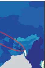
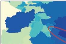
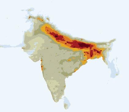
Comparing fine particulate matter (PM 2.5 ) exposure with expenditure statistics for districts

India reveals two large clusters (figure B5.2.1): First, a main cluster is grouped just at or below World Health Organization (WHO) Air Quality Interim Target 1 and includes a large group of districts with monthly expenditures of less than US$50 per capita. Second, a smaller cluster includes a number of districts that are well above the WHO Interim Target 1 standard, while having even lower levels of per capita expenditures. This smaller cluster represents the majority of districts over the WHO Interim Target 1 standard, showing that it is not just urban areas that experience high PM 2.5 exposure. Efforts to combat air pollution in South Asia must also contend with poverty in many of the most polluted districts in the region.
(box continued next page)
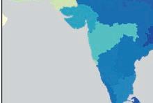
Airshedwide AQM will automatically include the abatement of more sources of air pollution. Current efforts in South Asia focus mainly on a small subset of emissions sources in cities: transportation, industry, and power plants. Once the focus broadens beyond cities, other emissions, which are particularly important in South Asia, can be reduced. These include emissions from solid fuel use in households, from brick kilns and ovens in other small industries, from agriculture, and from open burning of solid municipal waste. Further research is also needed to clarify the contribution of ammonia from open sewage systems, particularly in the central and eastern parts of the IGP.
Abatement costs for these additional sources of air pollution are relatively low, as illustrated in figure 5.2 with a marginal cost curve for the Indian state of Uttar Pradesh. This cost curve is based on the analysis underlying chapter 3. It shows the marginal costs of abatement opportunities in addition to existing policies. A number of options are identified that could reduce air pollution at negative cost. For brick kilns and waste management, the upfront investments are compensated for over their technical lifetimes by cost savings from efficiency improvements or revenues from the sale of side products. Additional reductions can be achieved with measures with marginal costs of less than €50 million per μg/m3 of PM2.5. These include, among others, stopping the open burning of agricultural residue and replacing traditional cremation practices with electric cremation. The largest single reduction potential is offered by universal access to clean cooking fuel (that is, electricity and liquefied petroleum gas) to eliminate solid fuel use in households.
In an airshedwide approach, the reduction of air pollution should be achieved as much as possible with joint targets. Learning from experience within an airshed can lead to joint policies. Such an approach is optimal and maintains a level playing field. Although additional policies are also needed to further reduce air pollution from power plants, traffic, and large industries, the three steps during this phase focus on the additional sources of pollution in an airshed.
Cleaner cookstoves are cost-effective, but implementation challenges remain. Reducing household air pollution by switching to cleaner cookstoves and using cleaner fuels for heating has been identified as one of the cost-effective measures for the region. Despite the effectiveness of clean cookstoves in improving health (see box 4.3), three main challenges to long-term adoption remain: (1) initial and maintenance costs, (2) knowledge and beliefs, and (3) compatibility with end users (Boudewijns et al. 2022). These challenges imply that economic support and information, in addition to adequate price signals, are key to achieving the adoption of clean fuel technology among mostly poor, rural households.
Agriculture in South Asia contributes to air pollution with the burning of fields and emissions of ammonia, mainly stemming from fertilizer use and manure management. The burning of fields results in high seasonal peaks in air pollution throughout the airsheds. Through chemical reactions in
ambient air, ammonia is a major contributor of PM2.5 in South Asia. The contributions from livestock to ammonia emissions could grow substantially over time. A study conducted in the United States suggests that livestock contributions to PM2.5 can be up to 20 percent of total emissions, depending on the region and climatic conditions (Hristov 2011).
Policies that eliminate, or at least reduce, the burning of fields can be a cost-effective measure for the region. Recent evidence from India shows that cash transfers as payments for ecosystem services can reduce agricultural burning by up to 80 percent (Jack et al. 2022), although Indonesia’s attempt to control agricultural burning through cash transfers has had mixed results (Falcon et al. 2022). Other examples of payments for sustainable agriculture, which may be adaptable to South Asia, have shown promising results in Latin America (Balseca et al. 2022).
Ultimately, the elimination of subsidies for the use of fertilizers and energy in agriculture should lead to more efficient fertilizer use in South Asia. However, in the short run, reforming these subsidies is challenging, given the complex political economy involved. Other interventions can successfully lower fertilizer use without compromising productivity. For example, Bangladesh’s simple rule-of-thumb training using colored leaf charts lowered fertilizer use by 8 percent without compromising yields, while China’s outreach program and workshops for smallholder farmers lowered nitrogen use by one-sixth and increased yields by about 11 percent (Damania et al. 2023).
Large-scale intensive livestock operations can prevent emissions through the scrubbing of ventilated air both into and out of animal housing areas. Various types of air purification systems are available, including combination filters that remove more than one pollutant (Guo et al. 2022). Abatement measures for animals not contained within housing include a switch to low-nitrogen feed, covered storage of manure, and application of manure on farms with technology designed to reduce ammonia emissions.
Less-polluting and more viable brick kiln technologies have been developed, but are slow in being adopted. Many brick kilns in South Asia are very small units using old, inefficient technologies. The inefficient combustion of coal and agricultural waste by these kilns generates particulate matter and carbon dioxide emissions. Cleaner and potentially more cost-effective technologies are already available. For example, existing kilns can be converted to improved “zig-zag” kilns that produce lower emissions and are more efficient in brick production. It is estimated that the upfront cost of installing zig-zag kilns can be recovered in two to three years given their superior productivity (Bhattacharjya 2017). However, the adoption rate of zig-zag kilns remains low.
Tailoring successful technology adoption programs for small firms and farmers to the context of brick kilns could help. Because brick kilns are so small, numerous, and spatially dispersed, a command-andcontrol approach to the diffusion of cleaner kilns is not feasible. Small firms in low- and middle-income countries are slow to adopt new technologies, even when those technologies appear to be cost-effective. The possible reasons for low adoption include credit constraints, a lack of information, and behavioral issues (Verhoogen 2021). Given the tiny size of kiln operations, the long payback period for zig-zag kilns, and their relative novelty, any of these constraints could be hampering their diffusion. Information campaigns and financial incentives can work, but only if their design is tailored to the context and targets the right constraint (Cirera, Frias, and Hill 2019). Research to better understand why zig-zag kilns are not being more widely adopted would help identify the best program design.
Municipal waste is a significant source of air pollution in South Asia. Many cities in South Asia have no waste collection, and even in cities with high collection rates, the segregation of waste and recycling is rare, which leads to open dumping or incineration of mixed waste (Ferronato and Torretta 2019). Uncontrolled incineration of waste contributes to many types of air pollution, including PM2.5,
heavy metals, and volatile organic compounds (Wiedinmyer, Yokelson, and Gullett 2014). Open dumping releases methane, a powerful greenhouse gas.
Municipal waste management is one of the most cost-effective potential interventions in the region. Modern disposal methods, including controlled incineration or chemical physical treatments, can provide significant air quality benefits at low cost. The most financially and environmentally friendly policies integrate multiple disposal processes: recycling, controlled incineration, composting for biodegradable waste, and managed landfills (Talang and Sirivithayapakorn 2021). By segregating waste in this way, each type can be optimally treated to reduce environmental impacts. For example, recycling programs are particularly important for plastics and electronic waste because of the toxic compounds released by the open incineration of these materials, and because precious or rare earth metals can be recovered from electronic components.
In the long run, the pricing of externalities through taxation or tradable emissions permits should play a central role in AQM. In the short run, mandated emissions standards, authorized filters or technologies, and bans on certain activities are the most effective methods for reducing air pollution. However, these methods come with disadvantages. Emissions standards reduce emissions per unit of economic activity, but they do not curb the total amount of polluting activity. Emissions standards also do not incentivize the private sector to develop technologies that reduce pollution to levels below the mandated standards. If pollution has a cost—in the form of a tax or the price of an emissions permit—total emissions are reduced more, and innovation is more stimulated. Taxation also has the advantage that AQM can be better integrated into other economic policies, meaning that synergies are better exploited, while trade-offs are more easily optimized. Tradable emissions permits facilitate the minimization of abatement costs across jurisdictions and across firms because those with lower abatement costs are automatically compensated for more-than-proportional reductions in pollution. Private and public funds to reduce air pollution will also be easier to mobilize in this third phase.
The taxation of activities that release pollutants will make cleaner technologies more competitive. Likewise, subsidies can encourage the use of clean industry and technologies that do not harm air quality. In both cases, such tax and subsidy policies might stimulate the development of domestic and regional markets for the manufacture of cleaner technologies and AQM infrastructure that drives down manufacturing costs and stimulates local operational and maintenance capacity.
Currently, most examples of taxes on air pollutants are found in developed economies. These taxes target primarily greenhouse gases or cover only one type of source (typically, large power plants or large firms in high-polluting industries). However, developing countries are increasingly experimenting with direct taxes on pollutants. For example, China has an environmental protection tax on PM2.5 precursors (sulfur dioxides [SO2], NOx, and soot), and Mexico imposed a carbon tax in 2014 that applies to carbon dioxide emissions from all sectors and covers all fossil fuels except natural gas. Meanwhile, in October 2021, Indonesia passed a law introducing a carbon tax on coal-fired power plants.
Several large countries provide subsidies to clean technologies. For example, the US Environmental Protection Agency’s Targeted Airshed Program gives grants to projects that reduce ambient PM2.5 pollution, including heavy-duty vehicle electrification, agricultural equipment replacement, alternatives to open burning, low-dust harvesting equipment, and reduction of road dust. The grant program is open to local and state pollution control authorities in targeted high-pollution areas across the country. Similar subsidy schemes are in place in the European Union and China. The Pradhan Mantri
Ujjwala Yojana (Prime Minister’s Lighting Scheme) program in India, which supports the use of liquefied petroleum gas, is another example of subsidizing cleaner technologies. Funding for such subsidies could come from reforming fossil fuel subsidies. Simulations show that such reforms would improve air quality and health (Rentschler, Klaiber, and Dorband 2021).
Market-based approaches to controlling emissions, such as airshedwide emissions trading systems (ETS), can have significant advantages. An airshed industrial ETS would establish an airshed-level cap on total industrial emissions from participating firms and allow them to trade emissions permits. Such an ETS gives firms throughout the airshed more flexibility to adjust their emissions and incentives to innovate. In addition, it automatically provides pecuniary compensation across jurisdictions for abatement efforts, which could facilitate least-cost emissions reduction in the airshed. Examples of such environmental markets that target air pollution include the United States’ Regional Clean Air Incentives Market program (introduced in 1994 to target SO2 and NOx), the Acid Rain Program (1995 to target SO2), and the NOx Budget Trading Program (introduced in 2003). More recently, the Regional Greenhouse Gas Initiative, a cooperative ETS among states along the eastern seaboard of the United States, enables cross-state cooperation and trade in emissions permits.
Recent evidence from a pilot ETS in India is encouraging. Until now, the experience and evidence base on ETS was wholly from selected high-income countries. This is no longer the case: a pilot particulate matter ETS was recently introduced in the state of Gujarat among 317 high-polluting plants in the airshed of a large industrial city. A critical precondition for this plan was the installation of robust monitoring systems in the participating firms. The pilot has been evaluated through a randomized control trial, which shows that it reduced emissions significantly and at low cost relative to the existing command-and-control regulation (Greenstone et al. 2022). Other ETS programs are being piloted or are under consideration in China, Mexico, Thailand, and Türkiye. These are promising developments that help prepare South Asia for the third phase of AQM. However, it is too early to assess the scalability and sustainability of such pilot programs.
An important advantage of using economic incentives is that they can mobilize funds from the private and public sectors for clean technologies. When the negative externalities of air pollution are incorporated into the price of technologies, the private sector finds investing in clean technologies to be profitable. The larger the area that imposes taxes, the easier it is for the private sector to invest at scale.
Economic instruments also generate government revenue that can be used to facilitate green innovation and address the distributional consequences of pollution abatement efforts. The funds from environmental taxes can play an important role in enticing cooperation within an airshed across jurisdictions. For example, the revenue generated from the Regional Greenhouse Gas Initiative has been used to fund climate-related programs, such as energy efficiency measures in residential and commercial facilities and renewable power generation, and to address equity impacts by providing direct electricity bill assistance (RGGI 2012). Several governments are linking revenues from carbon taxation to the funding of a “just transition” (World Bank 2022). For example, the European Union’s ETS revenues will feed into the Social Climate Fund, which cushions the impacts of the ETS on vulnerable households, micro enterprises, and transportation users.
Strong synergies exist between meeting cleaner air targets and meeting commitments to reduce greenhouse gas emissions (box 5.3). These synergies can help mobilize international funds that support pollution abatement or climate change mitigation. Some of these funds come from multilateral
The climate impact is an important side effect of air quality management. Although currently the reduction of greenhouse gases may not rank high on national policy agendas in South Asia, these reductions of carbon dioxide (CO2), black carbon, and methane (CH4) emissions would occur as a side effect of cost-effective strategies aimed at bringing ambient fine particulate matter (PM2.5) concentrations closer to the World Health Organization (WHO) Air Quality Interim Targets and gradually toward the WHO guideline values. The implementation of clean air strategies helps reduce CO2, black carbon, and methane. For example, reduction of concentrations to WHO Interim Target 1 (PM 2.5 level of 35 micrograms per cubic meter [µg/m3]) by 2030 and WHO Interim Target 4 (PM2.5 level of 10 µg/m3) by 2030 would reduce CO2 by 22 and 41 percent, black carbon by 81 and 89 percent, and methane by 21 and 28 percent, respectively (figure B5.3.1).
a.
b.
Waste
Agriculture
Nonroad machinery
Heavy-duty vehicles−diesel
Light-duty vehicles
Fuel production and distributio n
Industrial processes
Industrial combustion
Residentia l combustion
Power and heating plants
Waste
Agriculture
Nonroad machinery
Heavy-duty vehicles−diesel
Light-duty vehicles
Fuel production and distributio n
Industrial processes
Industrial combustion
Residentia l combustion
Power and heating plants
c.
Reductions in methane
Waste 0 20 40 60 80 100 120 140 Re lati ve to 2020 em is sions (percent)
Agriculture
Nonroad machinery
Light-duty vehicles
Fuel production and distributio n
Industrial processes
Industrial combustion
Residentia l combustion
Power and heating plants
development banks, scaling up existing programs that link financing to the achievement of AQM targets. Though still falling short of what is needed to avoid the most dangerous impacts of climate change, total global climate finance has steadily increased over the past decade, reaching US$632 billion in 2021 (Climate Policy Initiative 2021). Debt (of which 12 percent was low-cost or concessional debt) is its largest component (61 percent), followed by equity investments (33 percent) and grant finance (6 percent). Only 5 percent of global climate finance flowed into South Asia in 2021. Developing a climate change strategy that emphasizes the synergies with air pollution abatement and enacting reforms that strengthen data and institutions for AQM could help South Asian countries gain better access to international funds.
The road map presented above describes policy interventions that can achieve cleaner air in South Asia in a cost-effective way, but the path forward is far from easy. The analysis in this report shows that, from a technical point of view, direct economic gains from better air quality exceed the abatement costs needed to reduce air pollution. However, achieving these optimal solutions is not easy. It requires the building of better monitoring systems, more scientific capacity, and better coordination between governments. It requires behavioral change among farmers, small firms, and households. It requires experiments with greening tax systems and with tradable emissions permits. International experience has to be fine-tuned to the specific conditions in South Asia. It requires cross-border coordination across the South Asia region, which is far from straightforward, but the time is now to put conditions in place for such cross-border cooperation and the time is now to travel the road to cleaner air. The rewards of advancing on the road are high—the economic and social costs of a lack of progress are hard to overestimate.
Balseca, Esteban, Jose Antonio Cuesta, Richard Damania, Shenghui Feng, Jisung Moon, Jun Rentschler, Jason Russ, and Margaret Triyana. 2022. “The RISE Framework.” World Bank, Washington, DC.
Bhattacharjya, Souvik. 2017. “Assessing Social and Private Benefits and Costs for Improved Brick Production in Rajasthan.” Rajasthan Priorities, Copenhagen Consensus Center.
Boudewijns, Esther A., Maria Trucchi, Rianne M. J. J. van der Kleij, Debbie Vermond, Charlotte M. Hoffman, Niels H. Chavannes, Onno C. P. van Schayck, Bruce Kirenga, and Evelyn A. Brakema. 2022. “Facilitators and Barriers to the Implementation of Improved Solid Fuel Cookstoves and Clean Fuels in Low-Income and Middle-Income Countries: An Umbrella Review.” The Lancet Planetary Health 6 (7): e601–12.
Cirera, X., J. Frias, and J. Hill. 2019. “Instruments to Support Business Innovation: A Guide for Policy Makers and Practitioners.” Unpublished manuscript, World Bank, Washington, DC.
Climate Policy Initiative. 2021. “Global Landscape of Climate Finance 2021.” Climate Policy Initiative, San Francisco.
Damania, R., E. Balseca, C. de Fontaubert, J. Gill, K. Kim, J. Rentschler, J. Russ, and E. Zaveri. 2023. Detox Development: Repurposing Environmentally Harmful Subsidies. Washington, DC: World Bank.
Falcon, Walter, Gracia Hadiwidjaja, Ryan Edwards, Matthew Higgins, Rosamond Naylor, and Sudarno Sumarto. 2022. “Using Conditional Cash Payments to Prevent Land-Clearing Fires: Cautionary Findings from Indonesia.” Agriculture 12 (7): 1040.
Ferronato, Navarro, and Vincenzo Torretta. 2019. “Waste Mismanagement in Developing Countries: A Review of Global Issues.” International Journal of Environmental Research and Public Health 16 (6): 1060.
Greenstone, Michael, Rohini Pande, Anant Sudarshan, and Nicholas Ryan. 2022. “The Benefits and Costs of Emissions Trading: Experimental Evidence from a New Market for Industrial Particulate Emissions.” Working paper.
Guo, Li, Bo Zhao, Yingying Jia, Fuyang He, and Weiwei Chen. 2022. “Mitigation Strategies of Air Pollutants for Mechanical Ventilated Livestock and Poultry Housing—A Review.” Atmosphere 13 (3): 452. https://doi.org/10.3390/atmos13030452.
Hristov, A. N. 2011. “Contribution of Ammonia Emitted from Livestock to Atmospheric Fine Particulate Matter (PM2.5) in the United States.” Journal of Dairy Science 94 (6): 31303136.
Jack, B. Kelsey, Seema Jayachandran, Namrata Kala, and Rohini Pande. 2022. “Money (Not) to Burn: Payments for Ecosystem Services to Reduce Crop Residue Burning.” Working Paper 30690, National Bureau of Economic Research, Cambridge, MA.
Kummu, Matti, Maija Taka, and Joseph H. A. Guillaume. 2020. Data from Gridded global datasets for Gross Domestic Product and Human Development Index over 1990–2015, Dryad, Dataset. https://doi .org/10.5061/dryad.dk1j0
Rentschler, J., C. Klaiber, and I. Dorband. 2021. “Distributional and Health Co-Benefits of Fossil Fuel Subsidy Reforms.” Unpublished.
RGGI. 2012. “Regional Investment of RGGI CO2 Allowance Proceeds, 2011.” RGGI, Inc., New York.
Talang, R. P. N., and S. Sirivithayapakorn. 2021. “Environmental and Financial Assessments of Open Burning, Open Dumping and Integrated Municipal Solid Waste Disposal Schemes among Different Income Groups.” Journal of Cleaner Production 312: 127761.
Verhoogen, Eric. 2021. “Firm-Level Upgrading in Developing Countries.” Working Paper 29461, National Bureau of Economic Research, Cambridge, MA.
Wiedinmyer, Christine, Robert J. Yokelson, and Brian K. Gullett. 2014. “Global Emissions of Trace Gases, Particulate Matter, and Hazardous Air Pollutants from Open Burning of Domestic Waste.” Environmental Science and Technology 48 (16): 9523–30.
World Bank. 2022. State and Trends of Carbon Pricing 2022. Washington, DC: World Bank.

The World Bank Group is committed to reducing its environmental footprint. In support of this commitment, we leverage electronic publishing options and print-on-demand technology, which is located in regional hubs worldwide. Together, these initiatives enable print runs to be lowered and shipping distances decreased, resulting in reduced paper consumption, chemical use, greenhouse gas emissions, and waste.
We follow the recommended standards for paper use set by the Green Press Initiative. The majority of our books are printed on Forest Stewardship Council (FSC)–certified paper, with nearly all containing 50–100 percent recycled content. The recycled fiber in our book paper is either unbleached or bleached using totally chlorine-free (TCF), processed chlorine–free (PCF), or enhanced elemental chlorine–free (EECF) processes.
More information about the Bank’s environmental philosophy can be found at http://www.worldbank.org/corporateresponsibility
South Asia is home to 9 of the world’s 10 cities with the worst air pollution. Concentrations of fine particulate matter (PM2.5) in some of the region’s most densely populated and poor areas are up to 20 times higher than what the World Health Organization considers healthy (5 micrograms per cubic meter). This pollution causes an estimated 2 million premature deaths in the region each year and results in significant economic costs. Controlling air pollution is difficult without a better understanding of the activities that cause emissions of particulate matter. Air pollution travels long distances in South Asia and gets trapped in large “airsheds” that are shaped by climatology and geography. Striving for Clean Air identifies six major airsheds in the region and analyzes four scenarios for reducing air pollution with varying degrees of policy implementation and cooperation among countries.
The analysis shows that cooperation between different jurisdictions within an airshed is crucial, and a schematic road map with three phases is proposed. The phases in the road map may overlap when the rate of progress differs, depending on local circumstances. Phase 1 would improve monitoring and institutions; Phase 2 would introduce additional and joint targets for cost-effective abatement; and Phase 3 would mainstream air quality in the economy.
ISBN 978-1-4648-1831-8