28 minute read
Addressing a 10-µg/L Lead Trigger Level for a Blended Water Supply by Evaluating Alternative Corrosion Control Inhibitors—Paula


FWRJ Addressing a 10-µg/L Lead Trigger Level for a Blended Water Supply by Evaluating Alternative Corrosion Control Inhibitors
Paula Campesino and Steven J. Duranceau
The revised Lead and Copper Rule (LCR) was published in the Federal Register on Jan. 15, 2021, by the U.S. Environmental Protection Agency (EPA) and became effective on Dec. 16, 2021. It is anticipated that utilities will have to be compliant with this new law by Oct. 16, 2024. These revisions have motivated utilities to plan on how to best address these impending changes and determine how to effectively incorporate needed improvements, while managing existing corrosion programs already in place.
The University of Central Florida (UCF), through its department of civil, environmental, and construction engineering, has been performing corrosion control studies for water purveyors across the United States and its territories for over a decade. Recently, UCF was requested by the City of Sarasota Utilities Department (city) to investigate existing corrosion conditions (corrosion rates) of the system and forecast future possible needs if source waters were to change or existing unit operations were modified or replaced.
In this work, the use of precorroded linear polarization resistance (LPR) probes and coupons for conducting accurate and rapid corrosion control inhibitor screening studies is discussed.
A corrosion control testing rack apparatus using two identical parallel flow loops was designed and constructed to house mild steel, ductile iron, lead, and copper coupons used for weight-loss analysis, as well as mild steel, ductile iron, lead solder, and copper electrodes used for LPR analysis. Unlike other studies, coupons and electrodes were precorroded to simulate existing distribution system conditions. The city is interested in understanding its current water quality and the impacts to its distribution system corrosion chemistry, along with how modifications to its treatment process, for improved water quality, may influence corrosion rates.
This article provides an overview of a research project conducted for the city to evaluate the applicability and effectiveness of three blended phosphate chemical-based inhibitor formulations for the reduction of lead and copper corrosion rates. The corrosion test racks described herein were employed at the city’s facility. Both of these loops were fed by the city’s existing finished water supply, one of which was dosed with 1.6 mg/L of orthophosphate (with a varying polyphosphate dose based on the inhibitor’s ortho:poly ratio), after the initial stabilization period. Poststabilization, corrosion rates of the copper alloy decreased at varying degrees for the three inhibitor products tested.
One of the products resulted in a 60 percent decrease in the copper alloy corrosion rates. The lead/tin solder tested showed no statistically significant decrease or increase in the corrosion rate when exposed to the test condition, as compared to the existing condition. Of interest is the increase in the iron and mild steel alloy corrosion rates when an inhibitor was applied. Corrosion indices, such as the Langelier Saturation Index (LSI) and the Ryznar Stability Index (RI), were calculated for the existing condition, as well as the “future” condition. The “future” condition includes a reduced concentration of sulfate and total dissolved solids, among other parameters, as the city is assessing the feasibility of integrating nanofiltration into its current treatment process for one of its two well fields. A reduction in the amount of elemental sulfur is expected to increase lead corrosion since lead sulfide is insoluble.
Introduction
The corrosivity of a utility’s finished water may impact metals concentrations and water quality changes within its distribution system and at consumer taps. The recent EPA revision of the LCR maintains the current action levels for lead and copper, but introduces a lead trigger level of 10 parts per bil (ppb). The study presented investigates the existing corrosion conditions of the city’s finished water. This study is in response to the upcoming changes to the LCR and may result in the need for improvements and an analysis of how future water quality may affect the corrosion conditions in the distribution system.
Paula Campesino, MS, EI, is a graduate research assistant, and Steven J. Duranceau, Ph.D., P.E., is a professor with the department of civil, environmental, and construction engineering at the University of Central Florida in Orlando.
Regulatory Considerations
The LCR, promulgated by EPA in 1991, has an established action level of 0.015 mg/L for lead and 1.3 mg/L for copper (EPA, 2008). Potable water systems (PWS), must be compliant with the Lead and Copper Rule Revisions (LCRR) by October 2024, and are required to prepare for the following: a) Lead service line (LSL) inventory by January 2024 b) LSL replacement c) 5-liter sample draws for homes served by LSLs d) Sampling at schools and childcare facilities e) Expansion of public and community awareness and communication programs
With a greater focus on LSL replacement, sampling under these revisions prioritizes those sites served by LSLs (EPA, 2020); note that the city does not have LSLs and therefore (d) and (e) listed above stand out as the focus for the city moving forward. Along with these requirements comes the implementation of a new trigger level of 0.010 mg/L for lead. An exceedance of this concentration would “trigger” the start of corrosion control planning and increased treatment requirements. Corrosion control under the law can be undertaken through water chemistry changes or through the addition of a corrosion inhibitor.
Water Quality Considerations
The corrosion potential of finished waters is correlated to its water quality. A few parameters of importance, including pH, alkalinity, hardness, and disinfectant type (among several others) may affect the extent and type of corrosion present in a PWS distribution system. Of interest
in the work presented herein are the chloride and sulfate concentrations, usually characterized by the chloride-to-sulfate mass ratio (CSMR). It has been shown that a CSMR of less than 0.6 is preferred to reduce the corrosivity of the water in a distribution system and to reduce pitting potential (Edwards & Triantafyllidou, 2007). Changes in treatment, including the further removal of dissolved salts from raw water using membrane processes, such as nanofiltration (NF) or reverse osmosis (RO), can affect the CSMR and contribute to increased corrosion.
Common Corrosion Monitoring Techniques
There are several ways in which a utility may monitor the corrosion rates or the corrosion potential of its finished water. Traditional weightloss methods can be useful and practical for a less sophisticated way of getting insight on a finished water’s corrosivity. These traditional methods have the disadvantage of long wait periods with no immediate results. Pipe loops are also a common way to collect concentration data in a more-realistic setting. A disadvantage in these scenarios is the lack of control of certain parameters, such as temperature and reproducible water characteristics, since they are generally connected to a treatment facility for sufficient flow and pressure (Merkel & Pehkonen, 2006).
In recent times, electrochemical options provide instant feedback as to the current corrosion conditions. This niche of testing includes both electrochemical noise measurements and LPR. This study focuses on the use of LPR measurements to analyze the “instantaneous” corrosion rates of different metal alloys. Along with corrosion rates, the instrument can also measure the pitting index, which represents the ratio between the forward and reverse currents. This can indicate that there is asymmetry between the two electrodes installed and therefore suggests the potential for pitting; however, results of this asymmetry may manifest itself in ways other than pitting (Metal Samples, 2016).
Corrosion Indices
It is common to characterize or predict a water’s corrosion or scaling potential using indices, such as LSI, Calcium Carbonate Precipitation Potential (CCPP), RI, Larson-Skold Ratio (LSR), and more. While the applicability of these indices in real-world corrosion problems has not been completely successful, they will be used to compare different future treatment scenarios and how these changes can help predict corrosion control needs (McNeill & Edwards, 2002).
The LSI is simply a measure of the degree of calcium carbonate saturation (CaCO3) of a water. This index is commonly used in the industry and can inform on the potential of CaCO3 scaling. An LSI of greater than zero is considered to be a supersaturated solution (with a tendency to precipitate), an LSI of zero indicates this chemistry is in equilibrium, and one below zero indicates an undersaturated solution with the tendency for dissolution (Langelier, 1936). This measure is important in understanding aqueous corrosion chemistry because the formation of a CaCO3 precipitate may help mitigate corrosion by forming a protective coating on pipes.
The CCPP is another measure of how likely CaCO3 will precipitate out of solution. At a CCPP of zero, the solution is at equilibrium; above zero, it is oversaturated, with the CCPP value equivalent to the concentration of precipitant in mg/L, and below zero, it is undersaturated, equivalent to the amount of CaCO3 needed to reach oversaturation in mg/L (Mehl & Johannsen, 2017; Rossum & Merrill, 1983).
The RI is an index used to predict the “aggressiveness” of a water. At values less than 5.5, it is highly likely that scale forms, and beginning around a value of 7, the water is likely to be corrosive; after 8.5 it is considered increasingly aggressive and corrosive (Ryznar, 1944).
The LSR is the ratio between corrosive and inhibitory elements, i.e., the sum of chloride and sulfate versus the carbonate and bicarbonate (Larson & Skold, 1958). An LSR less than 0.8 is considered to be protective and may include film formation; between 0.8 and 1.2, the corrosive elements may hinder natural film formation; and a value greater than 1.2 indicates that corrosion is highly likely (Leitz & Guerra, 2013). The indices described herein, and their equations are summarized in Table 1.
Background
The city is supplied by two water sources, a brackish source and fresh water source, that contribute to its 12-mil-gal-per-day (mgd) maximum capacity. The first source is the Verna Wellfield (Verna), which consists of three separate wellfields (51 Lower Floridan aquifer wells). These waters are combined and aerated onsite through the implementation of tray aeration. Postaeration, the Verna water is dosed with chlorine for biological control prior to transport to the city’s water treatment facility (WTF) through a gravity-fed, 20-mi-long pipeline.
A portion of this aerated Verna water is treated through a cation exchange (CIX) process, while the remaining water is bypassed for blending. The second water source is the downtown wellfield, which consists of eight brackish water wells. This second well field is treated using RO, the permeate of which is aerated using packed towers and blended with the two Verna flows. During combination of the three streams, sodium hydroxide (NaOH) is added for pH adjustment, and the water is disinfected with sodium hypochlorite.
Table 2 summarizes the general water quality of the city’s finished water; note the high sulfate and total dissolved solids (TDS) content of this water (180 mg/L and 450 mg/L, respectively). Due to the new 0.010 mg/L lead trigger level in the revised LCR, the city requested that UCF perform a study to evaluate its current corrosion potential, as well as analyze its expected future water quality (associated with plant improvements and treatment additions) for corrosivity.
This part of the study analyzed the applicability of three different blended-phosphate corrosion inhibitor products on the corrosion rates of four metal alloys. Corrosion control test loops were built and operated by city and UCF staff at the city’s facilities over a period of about a year.
Materials and Methods
Corrosion Test Rack
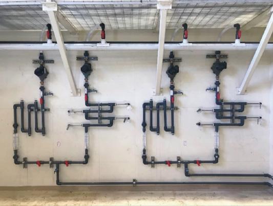
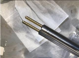
The analyses conducted within this research were done based on Standard Methods for the Examination of Water and Wastewater (Baird et al., 2017). The corrosion test racks employed at the city’s facility are presented in Figure 1. Examples of the metal coupons and the LPR electrodes used, provided by Metal Samples Co. Inc. (Munford, Ala.), are shown in Figure 2. The test rack consists of two parallel loops: one for existing conditions and the second for the test condition with inhibitor addition. Continued on page 18 Florida Water Resources Journal • February 2022 17
Test Rack Operation
The operation of the test rack was conducted similar to that done in previous work and includes a stabilization period for the corrosion rates of the metal alloys prior to dosing with inhibitor products (Duranceau et al., 2018). The test rack was continuously monitored for accurate dosing, pump operation, and flow rate consistency. Water quality field samples were collected at least twice weekly, grab samples were collected on a weekly basis, and LPR measurements were collected six days a week for a period of approximately three months per test.
The timer, which controls pump operation and test rack runtime, was programmed to run to reflect the typical household water use. The test rack ran for 6.5 hours per day between 6:30-9:30 a.m., 12-12:30 p.m., 5-8 p.m., and 12-12:30 a.m. The thirty-minute runtimes at noon and midnight were used to flush the system. The purpose of these flow and stagnant periods was to mimic a typical household, which has periods of stagnation.
Corrosion Monitoring Methods
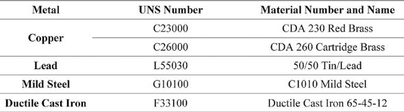
There were two monitoring methods used for the test rack: traditional weight-loss with metal coupons and LPR probe measurements. Table 3 presents the alloys used for this study.
The gravimetric method of using preweighed metal coupons, in addition to electrochemical methods, was included in this study as an inexpensive supplementary method of analysis. Metal coupons were placed in parallel racks, in order of nobility. After exposure, the coupons were carefully removed from the test rack, dried, and sent to Metal Samples Co. for postexposure analysis. This analysis included weight loss and pitting measurements. At the time of insertion and removal, the coupons were handled with nitrile gloves to prevent contamination due to handling.
Equation 1 provides the calculation to find the corrosion rate, given the parameters listed. Figure 3 provides an example of a coupon prior to exposure, after exposure, and after postcleaning. Equation 1
Where, W = weight loss (g) D = density of metal (g/cm3) A = area of test specimen (in2) T = exposure time (hours) K = 5.34 x 10⁵
The LPR is used to measure the in-situ “instantaneous” corrosion rate of a metal alloy. This is done by connecting the MS1500L to the LPR probes placed in the parallel test loops. The instrument runs approximately 20 millivolts (mV) through the electrodes, which sends a signal back and forth in each direction for the set length of time. Equation 2 and Equation 3 summarize the principals of the technology. The pitting index is also measured with this instrument and is simply the ratio between the forward and the reverse currents.
Continued on page 20
Table 2. Average Finished Water Quality
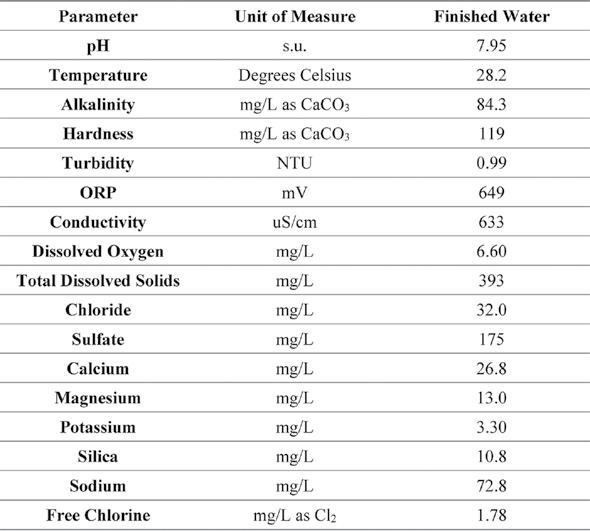
Table 3. Metal Alloys Tested Using Corrosion Test Rack Figure 1: Corrosion test racks at the City of Sarasota.
Equation 2
Where, ICORR = corrosion current generated by the flow of electrons E = equivalent weight of the corroding material (g) D = density of corroding metal (g/cm3) A = area of corroding electrode specimen (cm2) Equation 3
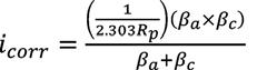
Where, i corr = corrosion current density (A/cm2) R p = polarization resistance (Ep/i) E p = polarization offset (<0.01 V) i = measured current density (A/cm2) βa = anodic Tafel constant βc = cathodic Tafel constant
Chemical Dosing
Three different inhibitors of varying orthophosphate and polyphosphate blends were tested. A goal of 1.6 +/- 0.1 mg/L of reactive phosphorus or orthophosphate dose (using Hach Method 8048) was to be achieved.
The following is a list and short description of each phosphate-based corrosion inhibitor tested: S Inhibitor A – 80 percent orthophosphate and 20 percent polyphosphate blend S Inhibitor B – 75 percent orthophosphate and 25 percent polyphosphate blend S Inhibitor C – 70 percent orthophosphate and 30 percent polyphosphate blend
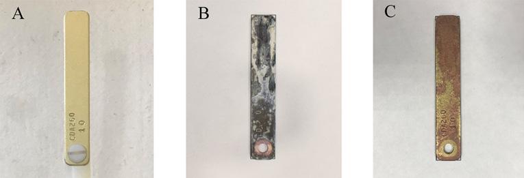
Figure 3. Example of a copper metal coupon a) pre-exposure, b) postexposure, and c) postcleaning.
Statistical Analysis
In order to statistically analyze the applicability of each inhibitor, the Wilcoxon Signed Rank Test and the Wilcoxon Rank Sum Test were used, based on Wysock et al. (1995) procedures. The prestabilization phase was statistically analyzed using a two-tailed test, which indicates whether both sides of the test rack are corroding at the same rate for each metal alloy. The inhibitor effectiveness was conducted with a one-tailed test, which analyzes if the effects of the inhibitor are of significance; the one-tailed test is presented in Equation 4 and the two-tailed test is presented in Equation 5. A 95 percent (α = 0.05) confidence interval is used to determine the critical region for both tests.
The results presented herein are supported by statistical analysis using the Wilcoxon Rank Sum Test and the Wilcoxon Signed Rank Test. Prior to analysis using these methods, outliers were removed from the dataset.
Equation 4
Equation 5
Results and Discussion
Linear Polarization Resistance Corrosion Rates
Lead Alloy
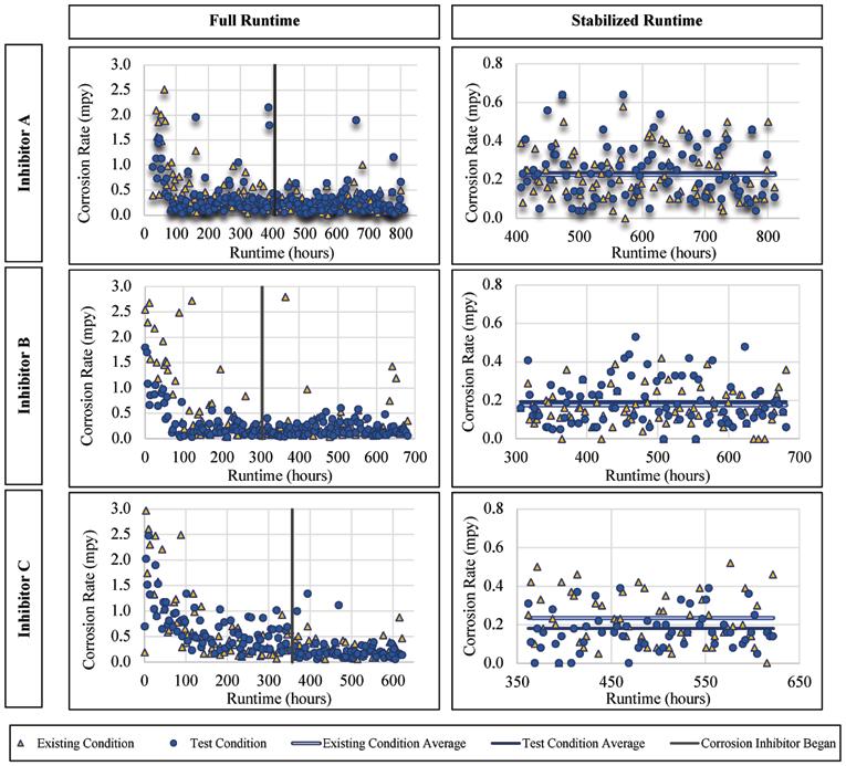
For the lead-tin alloy there were no statistically significant improvements or worsening of the corrosion rates when exposed to Inhibitors A and B, with slight improvement when exposed to Inhibitor C. The corrosion
rates versus runtime are presented for Inhibitor A, B, and C in Figure 4. The average corrosion rate of the lead for Inhibitor A was 0.23 mils penetration per year (mpy), a statistically insignificant change from the 0.24 mpy without inhibitor addition (a mil is a thousandth of an in.). The average corrosion rate of the alloy when exposed to Inhibitor B was 0.19 mpy as compared to 0.17 mpy without the inhibitor addition. When exposed to Inhibitor C the lead corrosion rate was 0.16 mpy, compared to 0.23 mpy without inhibitor. In general, the lead alloy was unaffected by the addition of a corrosion inhibitor based on this LPR data, except when exposed to Inhibitor C.
Copper Alloy
For the copper alloy there was a statistically significant improvement of the corrosion rates for the three inhibitor products, as supported by the Wilcoxon Rank Sum Test and the Wilcoxon Signed Rank Test. The corrosion rates versus runtime are presented for Inhibitor A, B, and C in Figure 5. The average corrosion rate of the copper alloy when exposed to Inhibitor A was 0.52 mpy, versus 1.4 mpy without inhibitor addition. This accounts for an over 60 percent reduction in the average copper corrosion rate. The average corrosion rate of the alloy when exposed to Inhibitor B was 0.54 mpy as compared to 1.16 mpy without the inhibitor addition, a 53 percent reduction. Similarly, the addition of Inhibitor C lowered the average corrosion rate to 0.49 mpy as compared to 1.01 mpy without inhibitor addition.
Mild Steel Alloy
For the mild steel there was a visible increase of the corrosion rates for each inhibitor post-stabilization, i.e., during inhibitor addition. The mild steel corrosion rates versus runtime are presented for Inhibitor A, B, and C in Figure 6. The average corrosion rate when exposed to Inhibitor A was 6.67 mpy, compared to 4.13 mpy without inhibitor addition. Since these values cannot be directly compared (because the two loops were not corroding at the same rate prior to inhibitor addition) they were normalized based on their corresponding pre-inhibitor stable average, which gives values of 0.995 and 1.21 for the existing and test conditions, respectively.
From these normalized values, there is an overall increase of mild steel corrosion with the addition of Inhibitor A. The average corrosion rate of the alloy when exposed to Inhibitor B was 6.47 mpy as compared to 5.24 mpy without the inhibitor addition, with normalized values of 1.10 and 1.06, respectively. When exposed to Inhibitor C the average corrosion rate was 6.60 mpy compared to 5.11 mpy without inhibitor. Continued on page 22
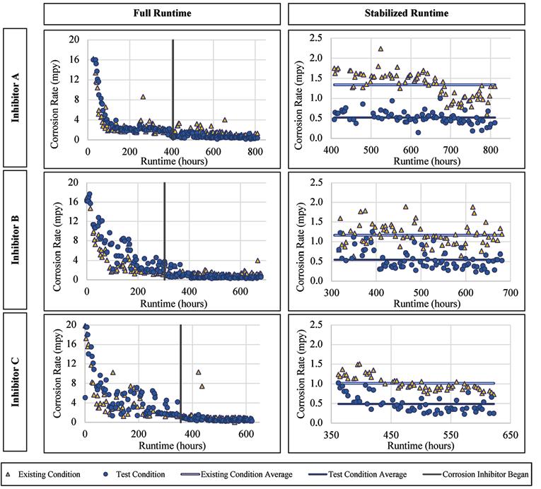
Figure 5. Corrosion rate versus runtime for copper when exposed to the inhibitor products.
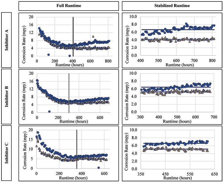
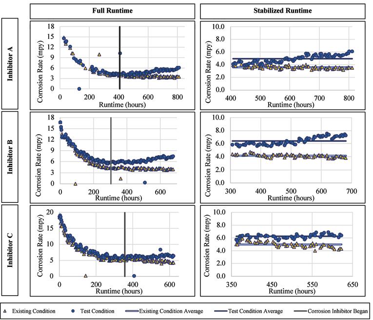
Figure 7. Corrosion rate versus runtime for ductile iron when exposed to the inhibitor products.
Figure 8. Pitting index versus runtime for lead exposed to inhibitor products. Continued from page 21 The normalized values for these were 1.15 and 1.10, respectively.
Ductile Iron Alloy
Similar to the mild steel, there was a visible increase in the ductile iron corrosion rates for each inhibitor, post-stabilization/postinhibitor addition. The ductile iron corrosion rates versus runtime are presented for Inhibitor A, B, and C in Figure 7. The average corrosion rate when exposed to Inhibitor A was 4.95 mpy as compared to 3.95 mpy without inhibitor addition. When normalized based on the preinhibitor stable average, the values are 0.91 and 1.12 for the existing and test conditions, respectively. These normalized values show an overall increase of ductile iron corrosion with the addition of Inhibitor A. The average corrosion rate of the alloy when exposed to Inhibitor B was 6.41 mpy as compared to 4.15 mpy without the inhibitor addition, with normalized values of 1.17 and 0.93, respectively. When exposed to Inhibitor C the average corrosion rate was 6.26 mpy compared to 4.99 mpy without inhibitor. The normalized values for these were 1.14 and 0.97, respectively.
Linear Polarization Resistance Pitting Index
Lead Alloy
Like with the corrosion rates, the lead alloy was not affected by the addition of a blended phosphate corrosion inhibitor regarding the pitting index measured. When Inhibitor A was being dosed, the pitting index averaged 0.98 with a standard deviation of 0.66, compared to 0.93 and 0.59, respectively, for the existing condition. When Inhibitor B was being dosed, the pitting index averaged 1.43 with a standard deviation of 1.22, compared to 1.32 and 1.15, respectively, for the existing condition. When exposed to Inhibitor C the pitting index averaged 1.32 with a standard deviation of 1.10, compared to 1.41 and 1.00, respectively, without inhibitor addition. Figure 8 presents the pitting index for lead during the inhibitor-addition phase.
Copper Alloy
The copper alloy showed a decrease in the pitting index with the addition of a blended phosphate corrosion inhibitor. When Inhibitor A was dosed, the pitting index averaged 0.88 with a standard deviation of 0.76, compared to 2.00 and 1.48, respectively, for the existing condition. When Inhibitor B was dosed, the pitting index averaged 0.32 with a standard deviation of 0.22, compared to 1.40 and 1.06, respectively, for the existing condition. When exposed to Inhibitor C the average pitting index was 0.50 with a standard deviation of 0.38, compared to 0.85
and 0.46, respectively, for the existing condition. Figure 9 presents the pitting index for copper during the inhibitor-addition phase.
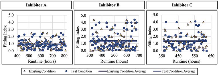
Mild Steel Alloy
The mild steel alloy was not seemingly affected by the addition of a blended phosphate corrosion inhibitor regarding the pitting index measured. When Inhibitor A was being dosed, the pitting index averaged 1.00 with a standard deviation of 0.0, compared to 0.98 and 0.12, respectively, for the existing condition. When Inhibitor B was being dosed, the pitting index averaged 0.95 with a standard deviation of 0.07, compared to 1.02 and 0.08, respectively, for the existing condition. Similar trends were observed when exposed to Inhibitor C where the mild steel had an average pitting index of 1.00 and 0.97 without inhibitor addition. Figure 10 presents the pitting index for mild steel during the inhibitor-addition phase.
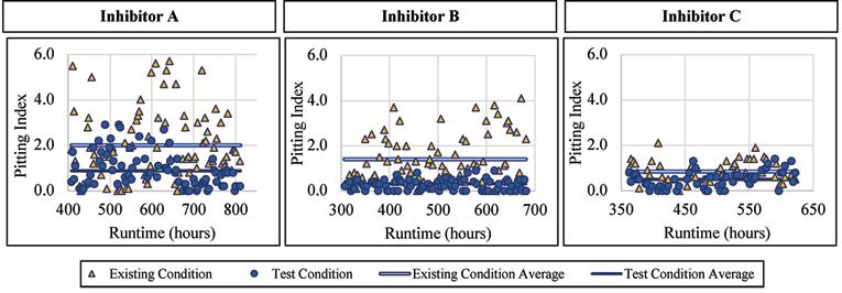
Ductile Iron Alloy
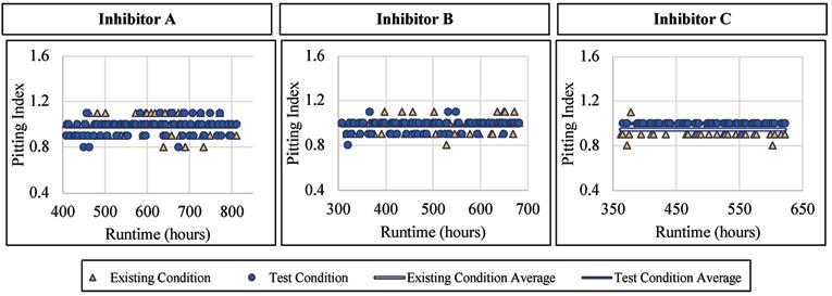
The ductile iron alloy was not affected by the addition of a blended phosphate corrosion inhibitor regarding the pitting index measured. When Inhibitor A was dosed, the pitting index averaged 0.98 with a standard deviation of 0.07, compared to 0.98 and 0.08, respectively, for the existing condition. When Inhibitor B was dosed, the pitting index averaged 0.98 with a standard deviation of 0.05, compared to 0.98 and 0.06, respectively, for the existing condition. Similarly, when exposed to Inhibitor C, the ductile iron had an average pitting index of 0.97, and 0.95 without inhibitor addition. Figure 11 presents the pitting index for ductile iron during the inhibitor-addition phase.
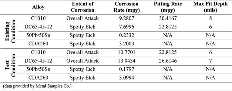
Gravimetric Method: Weight-Loss Results
Also included in this study was the analysis of metal coupons inserted in the corrosion test rack. Postexposure analyses of the coupons were conducted by Metal Samples Co. The corrosion rates of the alloys tested, per the results of these analyses, are presented in Tables 4, 5, and 6. These results show increased corrosion rates in the mild steel and ductile iron coupons when inhibitor products were used, similar to that shown by the LPR measurements. The corrosion rate of the lead and copper metal coupons decreased with the addition of the corrosion inhibitors.
Pitting was present at the same rate in both the existing and test conditions for the ductile iron coupons, when exposed to Inhibitor A. Pitting, when exposed to Inhibitor B, increased for the mild steel and ductile iron, compared to the existing condition. When exposed to Inhibitor C, there was an increase in pitting for the ductile iron Continued on page 24
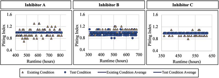
Figure 10. Pitting index versus runtime for mild steel when exposed to inhibitor products.
Figure 11. Pitting index versus runtime for ductile iron when exposed to inhibitor products.
Table 4. Corrosion Rate and Pitting Analysis of Metal Coupons – Inhibitor A
Table 5. Corrosion Rate and Pitting Analysis of Metal Coupons – Inhibitor B
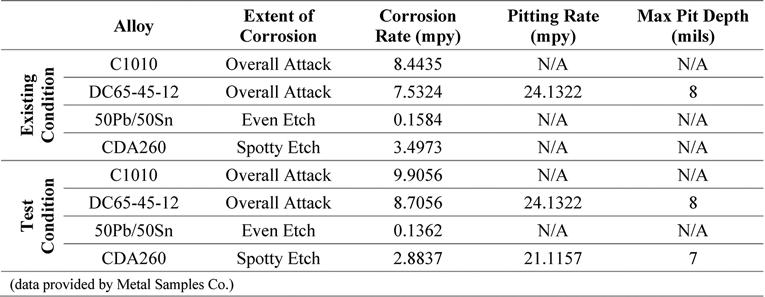
Continued from page 23 coupon, and a decrease for the mild steel coupon. There was no discernable pitting for the copper coupons, except when exposed to Inhibitor A, suggesting this inhibitor is incompatible regarding the potential for copper pitting. Other studies have shown that incompatibility of phosphatebased inhibitors can cause an increase in copper corrosion rates (Duranceau et al., 2018). The lead coupons showed no signs of pitting in the conditions tested.
Model Predictions of Distributed Water for the Future
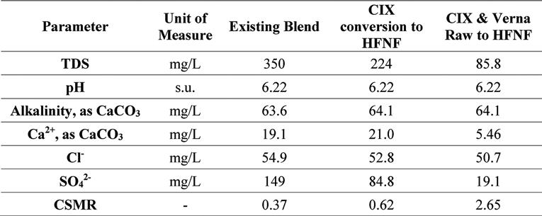
The future finished water is based on improvements to the Verna groundwater supply treatment. Currently, the average annual daily flow (AADF) includes 4.5-mgd RO permeate production, 1.2-mgd CIX process production, and 1.2-mgd Verna Raw bypass water. The treatment scenarios considered in this evaluation are a) replacement of the CIX process with a hollow fiber nanofiltration (HFNF), i.e., 1.2-mgd HFNF permeate production, and b) replacement of CIX process with HFNF and removal of the raw Verna bypass, i.e., 2.4-mgd HFNF permeate production. The pertinent water quality for each of these scenarios is presented in Table 7.
Shown in the bar charts in Figure 12 and Figure 13 are the results of the corrosion and scaling indices calculated for each of the scenarios, using the Tetra Tech RTW Model (2011). As a point of reference, the existing finished water quality has a CSMR of approximately 0.17. At CSMRs below 0.5, galvanic corrosion of lead is said to be minimal (Edwards & Triantafyllidou, 2007). Based on the results of these modeled indices, it is expected that the corrosivity of the water will be higher with increased treatment of the Verna wellfields, which is in part due to the removal of TDS, calcium, and sulfate.
Conclusions
The results of this research show that a blended phosphate inhibitor would be helpful in reducing copper corrosion rates; however, the majority of the inhibitors tested had no significant effects on the corrosion rate of lead when measuring the instantaneous rates using LPR techniques. Still, the gravimetric method using metal coupons showed a 14 percent, 25
Table 6. Corrosion Rate and Pitting Analysis of Metal Coupons – Inhibitor C
Table 7. Water Quality Values Used in Model, With an Assumed 65, 82, 85, and 90 Percent Rejection of Chloride, Total Dissolved Solids, Calcium, and Sulfate, Respectively, When Using Hollow Fiber Nanofiltration*
*Assumptions based on best-performing membranes tested at the bench scale from work performed by Yonge (2016) percent, and 23 percent decrease in the overall corrosion rate of lead when exposed to Inhibitor A, B, and C, respectively. The average pitting index of the copper alloy was also reduced when a blended phosphate inhibitor was used. Assessing the pitting found on the metal coupons, there are no signs of pitting, both in the existing and test conditions, except for when Inhibitor A was used.
Of note are the increased LPR corrosion rates of both mild steel and ductile iron when exposed to the blended phosphate products, which is further supported by the corrosion rates calculated using the gravimetric method. These results indicate that the use of a blended phosphate product may be beneficial for meeting the regulations set forth by the LCR and LCRR; however, it may cause concern regarding corrosion of other metals that are not lead and copper.
Based on the indices calculated for the current and future process waters, it is expected that the corrosivity of the water will most likely degrade with further treatment of the Verna water. For this reason, it was recommended that the city plan for the addition of a corrosion control inhibitor to the finished water to provide additional corrosion control benefits for the “future” planned water supply.
Next Steps
Due to the anticipated further treatment of the Verna water, the next step in this study is to test the effects of different Verna treatment options and blends on the corrosivity of their finished water. This further treatment is expected to reduce the water’s sulfate and TDS content. Because of this, it is anticipated that the corrosivity of the water will also increase, based on the CSMR principle and other indices.
The study will include bench-scale treatment of the Verna water, blending with the current RO aerated permeate and/or CIX process water. A novel flow-through coupon test rack will be used to analyze the corrosivity of this future finished water, with and without a corrosion inhibitor, and will allow for the measurement of metals concentrations and gravimetric analysis, but not LPR corrosion rates.
Acknowledgments
This work was funded by the City of Sarasota Utilities Department (UCF Project 1620-8A15). Dr. S.J. Duranceau served as the principal investigator. The authors acknowledge the City of Sarasota staff, especially Bill Reibe, Verne Hall, Pedro Perez, and Tomasz Torski, for their help and support. The authors would also like to acknowledge and thank the city operators who helped in coordinating the work and
collecting data, without which this work would not have been possible. The efforts of UCF Water Quality Engineering Research Group were greatly appreciated and contributed to the success of this research. Any opinion, findings, conclusions, or recommendations expressed in this material are those of the authors and do not necessarily reflect the views of UCF, nor serve as an endorsement of any company, product, equipment, or material identified herein.
References
• Baird, R. B., Eaton, A. D., & Rice, E. W. (2017).
Standard Methods for the Examination of
Water and Wastewater (23rd ed.). Washington:
American Public Health Association,
American Water Works Association, Water
Environment Federation. • Duranceau, S., Rodriguez, A. B., Higgins, C.,
Wilder, R. J., Myers-O Farrell, S., Black, S. J., & Yoakum, B. A. (2018). Use of Precorroded
Linear Polarization Probes and Coupons for Conducting Corrosion Control Studies.
Florida Water Resources Journal. • Edwards, M., & Triantafyllidou, S. (2007).
Chloride-to-sulfate mass ratio and lead leaching to water. Journal AWWA, 99(7), 96-109. doi:https://doi.org/10.1002/j.1551-8833.2007. tb07984.x. • Langelier, W. F. (1936). The Analytical Control of Anti-Corrosion Water Treatment. Journal
AWWA, 28(10), 1500-1521. doi:https://doi. org/10.1002/j.1551-8833.1936.tb13785.x. • Larson, T. E., & Skold, R. V. (1958). Laboratory
Studies Relating Mineral Quality of Water To
Corrosion of Steel and Cast Iron. Corrosion, 14(6), 43-46. doi:10.5006/0010-9312-14.6.43. • Leitz, F., & Guerra, K. (2013). Water Chemistry
Analysis for Water Conveyance, Storage, and
Desalination Projects. Denver, Colo.: U.S.
Department of the Interior. • McNeill, L. S., & Edwards, M. (2002). The
Importance of Temperature in Assessing Iron
Pipe Corrosion in Water Distribution Systems.
Environmental Monitoring and Assessment, 77(3), 229-242. doi:10.1023/A:1016021815596. • Mehl, V., & Johannsen, K. (2017). Calculating chemical speciation, pH, saturation index and calcium carbonate precipitation potential (CCPP) based on alkalinity and acidity using
OpenModelica. Journal of Water Supply:
Research and Technology - Aqua, 67(1), 1-11. doi:10.2166/aqua.2017.103. • Merkel, T. H., & Pehkonen, S. O. (2006). General corrosion of copper in domestic drinking water installations: scientific background and mechanistic understanding. Corrosion
Engineering, Science and Technology, 41(1), 21-37. doi:10.1179/174327806X94009. • Metal Samples, I. (2016). MS1500L LPR Data
Logger User’s Manual. Metal Samples Co.,
Munford, Ala. Retrieved from https://www. alspi.com/manuals/ms1500Lmanual.pdf. • Rossum, J. R., & Merrill, D. T. (1983). An evaluation of the calcium carbonate saturation indexes. Journal - American Water Works
Association, 75(2), 95-100. Retrieved from http://www.jstor.org/stable/41271574. • Ryznar, J. W. (1944). A New Index for Determining Amount of Calcium
Carbonate Scale Formed by a Water. Journal
AWWA, 36(4), 472-483. doi:https://doi. org/10.1002/j.1551-8833.1944.tb20016.x. • Tetra Tech, I. (2011). Tetra Tech (RTW) Model for Water Process and Corrosion Chemistry (Version 2.0) [CD-ROM]: American Water
Works Association. • USEPA (2008). Lead and Copper Rule: A Quick
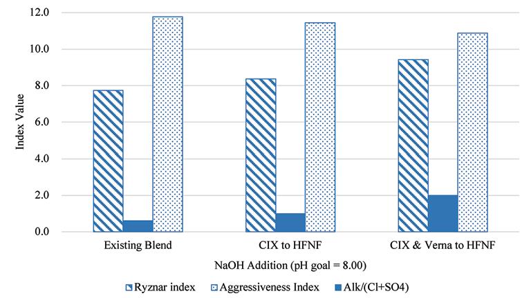
Figure 12. Results of corrosion indices calculated for the existing blend ratio at average annual daily flow production and the two future treatment scenarios.
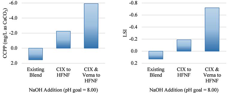
Figure 13. Calcium carbonate precipitation potential (left) and the Langelier Saturation Index (right) for the existing blend ratio at average annual daily flow production and the two future treatment scenarios.
Reference Guide. Washington, D.C., Office of
Water. • USEPA (2020). Reference Guide for Public
Water Systems, Lead and Copper Rule
Comparison. Retrieved from https://www.epa. gov/sites/default/files/2020-12/documents/ reference_guide_for_pwss_12.21.20.pdf. • Wysock, B. M., Sandvig, A. M., Schock,
M. R., Frebis, C. P., & Prokop, B. (1995).
Statistical procedures for corrosion studies.
Journal AWWA, 87(7), 99-112. doi:https://doi. org/10.1002/j.1551-8833.1995.tb06397.x. • Yonge, D. (2016). Modeling Mass Transfer and
Assessing Cost and Performance of a Hollow
Fiber Nanofiltration Membrane Process. (Doctor of Philosophy [Ph.D.]). University of
Central Florida. College of Engineering and
Computer Science, Retrieved from http://purl. fcla.edu/fcla/etd/CFE0006549. S


