


Physics for the IB Diploma Together with IB teachers Seventhedition Digital Access MULTI-COMPONENT SAMPLE Executive Preview SAMPLE Original material © Cambridge University Press & Assessment 2023. This material is not final and is subject to further changes prior to publication. Any references or material related to answers, grades, papers or examinations are based on the opinion of the author(s)
Original material © Cambridge University Press & Assessment 2023. This material is not final and is subject to further changes prior to publication. Any references or material related to answers, grades, papers or examinations are based on the opinion of the author(s)
SAMPLE
Dear Teacher,
Welcome to the new edition of our Physics for the IB Diploma series, providing full support for the new course for examination from 2025. This new series has been designed to exibly meet all of your teaching needs, including extra support for the new assessment. This preview will help you understand how the coursebook, the workbook and the teacher’s resource work together to best meet the needs of your classroom, timetable and students. This Executive Preview contains sample content from the series, including:
• A guide explaining how to use the series
• A guide explaining how to use each resource
In developing this new edition, we carried out extensive global research with IB Physics teachers – through lesson observations, interviews and work on the Cambridge Panel, our online teacher research community. Teachers just like you have helped our experienced authors shape these new resources, ensuring that they meet the real teaching needs of the IB Physics classroom.
The coursebook has been speci cally written to support English as a second language learners with key subject words, glossary de nitions in context and accessible language throughout. We have also provided new features that help with active learning, assessment for learning and student re ection. Numerous exam-style questions with answers in the digital coursebook, which accompanies the print coursebook, ensure your students feel con dent approaching the assessment and have all the tools they need to succeed in their examination. Core to the series is the brand-new digital teacher’s resource. It will help you support your learners and con dently teach to the new IB Physics guide, whether you are new to teaching the subject or more experienced. For each topic there are lesson ideas and activities, common misconceptions to look out for, worksheets, PowerPoint presentations, answers to the coursebook, extra wrap-up activities and more. Also included is a practical guide to help your students develop their academic writing.
Please take ve minutes to nd out how our resources will support you and your learners. To view the full series, you can visit our website or speak to your local sales representative. You can nd their contact details here:
cambridge.org/gb/education/ nd-your-sales-consultant
Best wishes,
Micaela Inderst
Senior Commissioning Editor for the IB Diploma Cambridge University Press


SAMPLE Original material © Cambridge University Press & Assessment 2023. This material is not final and is subject to further changes prior to publication. Any references or material related to answers, grades, papers or examinations are based on the opinion of the author(s)
How to use this series


This suite of resources supports students and teachers of the IB Physics Diploma course. All of the books in the series work together to help students develop the necessary knowledge and scienti c skills required for this subject.


The coursebook with digital access provides full coverage of the latest IB Physics Diploma course.


It clearly explains facts, concepts and practical techniques, and uses real world examples of scienti c principles. A wealth of formative questions within each chapter help students develop their understanding, and own their learning. A dedicated chapter in the digital coursebook helps teachers and students unpack the new assessment, while exam-style questions provide essential practice and self-assessment. Answers are provided on Cambridge GO, supporting self-study and home-schooling.
The workbook with digital access builds upon the coursebook with digital access with further exercises and exam-style questions, carefully constructed to help students develop the skills that they need as they progress through their IB Physics Diploma course. The exercises also help students develop understanding of the meaning of various command words used in questions, and provide practice in responding appropriately to these.
The Teacher’s resource supports and enhances the coursebook with digital access and the workbook with digital access. This resource includes teaching plans, overviews of required background knowledge, learning objectives and success criteria, common misconceptions, and a wealth of ideas to support lesson planning and delivery, assessment and differentiation. It also includes editable worksheets for vocabulary support and exam practice (with answers) and exemplar PowerPoint presentations, to help plan and deliver the best teaching.
PHYSICS FOR THE IB DIPLOMA: COURSEBOOK 4
Physics
COURSEBOOK Together Seventhedition Digital Access Physics
the IB Diploma WORKBOOK Together with IB teachers Secondedition Digital Access Second edition Physics
Diploma Together with IB teachers Digital Teacher’s Resource
for the IB Diploma
for
for the IB
SAMPLE Original material © Cambridge University Press & Assessment 2023. This material is not final and is subject to further changes prior to publication. Any references or material related to answers, grades, papers or examinations are based on the opinion of the author(s)


Physics for the IB Diploma COURSEBOOK Together with IB teachers Seventhedition Digital Access SAMPLE Original material © Cambridge University Press & Assessment 2023. This material is not final and is subject to further changes prior to publication. Any references or material related to answers, grades, papers or examinations are based on the opinion of the author(s)
PHYSICS FOR THE IB DIPLOMA: COURSEBOOK 6 Contents How to use this series vi How to use this book vii Unit A Space, time and motion 1 1 Kinematics 2 1.1 Displacement, distance, speed and velocity 3 1.2 Uniformly accelerated motion: the equations of kinematics 7 1.3 Graphs of motion 16 1.4 Projectile motion 20 2 Forces and Newton’s laws 30 2.1 Forces and their direction 31 2.2 Newton’s laws of motion 40 2.3 Circular motion 53 3 Work, energy and power 63 3.1 Work 64 3.2 Conservation of energy 72 3.3 Power and efficiency 80 3.4 Energy transfers 82 4 Linear momentum 87 4.1 Newton’s second law in terms of momentum 88 4.2 Impulse and force–time graphs 90 4.3 Conservation of momentum 93 4.4 Kinetic energy and momentum 96 4.5 Two-dimensional collisions 100 5 Rigid body mechanics 105 5.1 Kinematics of rotational motion 106 5.2 Rotational equilibrium and Newton’s second law 109 5.3 Angular momentum 122 6 Relativity 128 6.1 Reference frames and Lorentz transformations 129 6.2 Effects of relativity 137 6.3 Spacetime diagrams 146 Unit B The particulate nature of matter 159 7 Thermal energy transfers 160 7.1 Particles, temperature and energy 161 7.2 Specific heat capacity and change of phase 165 7.3 Thermal energy transfer 172 8 The greenhouse effect 179 8.1 Radiation from real bodies 180 8.2 Energy balance of the Earth 184 9 The gas laws 192 9.1 Moles, molar mass and the Avogadro constant 193 9.2 Ideal gases 195 9.3 The Boltzmann equation 203 10 Thermodynamics 209 10.1 Internal energy 210 10.2 The first law of thermodynamics 215 10.3 The second law of thermodynamics 222 10.4 Heat engines 228 11 Current and circuits 236 11.1 Potential difference, current and resistance 237 11.2 Voltage, power and emf 243 11.3 Resistors in electrical circuits 246 11.4 Terminal potential difference and the potential divider 259 SAMPLE Original material © Cambridge University Press & Assessment 2023. This material is not final and is subject to further changes prior to publication. Any references or material related to answers, grades, papers or examinations are based on the opinion of the author(s)
7 Contents Unit C Wave behaviour 269 12 Simple harmonic motion 270 12.1 Simple harmonic oscillations 271 12.2 Details of simple harmonic motion 279 12.3 Energy in simple harmonic motion 285 12.4 More about energy in SHM 287 13 The wave model 292 13.1 Mechanical pulses and waves 293 13.2 Transverse and longitudinal waves 296 13.3 Electromagnetic waves 304 13.4 Waves extension 305 14 Wave phenomena 307 14.1 Reflection and refraction 308 14.2 The principle of superposition 314 14.3 Diffraction and interference 317 14.4 Single-slit diffraction 324 14.5 Multiple slits 328 15 Standing waves and resonance 335 15.1 Standing waves 336 15.2 Standing waves on strings 337 15.3 Standing waves in pipes 340 15.4 Resonance and damping 346 16 The Doppler effect 352 16.1 The Doppler effect at low speeds 353 16.2 The Doppler effect for sound 357 Unit D Fields 363 17 Gravitation 364 17.1 Newton’s law of gravitation 365 17.2 Gravitational potential and energy 372 17.3 Motion in a gravitational field 379 18 Electric and magnetic fields 390 18.1 Electric charge, force and field 391 18.2 Magnetic field and force 401 18.3 Electrical potential and electrical potential energy 412 19 Motion in electric and magnetic fields 422 19.1 Motion in an electric field 423 19.2 Motion in a magnetic field 427 20 Electromagnetic induction 434 20.1 Electromagnetic induction 435 20.2 Generators and alternating current 449 Unit E Atomic, quantum and nuclear physics 455 21 Atomic physics 456 21.1 The structure of the atom 457 21.2 Quantisation of angular momentum 463 22 Quantum physics 468 22.1 Photons and the photoelectric effect 469 22.2 Matter waves 479 23 Nuclear physics 484 23.1 Mass defect and binding energy 485 23.2 Radioactivity 492 23.3 Nuclear properties and the radioactive decay law 500 24 Nuclear fission 512 24.1 Nuclear fission 513 25 Nuclear fusion and stars 520 25.1 Nuclear fusion 521 25.2 Stellar properties and the Hertzsprung–Russell diagram 522 25.3 Stellar evolution extension 529 Glossary 535 Index 000 Acknowledgements 000 SAMPLE Original material © Cambridge University Press & Assessment 2023. This material is not final and is subject to further changes prior to publication. Any references or material related to answers, grades, papers or examinations are based on the opinion of the author(s)
Original material © Cambridge University Press & Assessment 2023. This material is not final and is subject to further changes prior to publication. Any references or material related to answers, grades, papers or examinations are based on the opinion of the author(s)
SAMPLE
How to use this book
Throughout this book, you will find lots of different features that will help your learning. These are explained below.
UNIT INTRODUCTION
A unit is made up of a number of chapters. The key concepts for each unit are covered throughout the chapters.
LEARNING OBJECTIVES
Each chapter in the book begins with a list of learning objectives. These set the scene for each chapter, help with navigation through the coursebook and indicate the important concepts in each topic.
• A bulleted list at the beginning of each section clearly shows the learning objectives for the section.
GUIDING QUESTIONS
This feature contains questions and activities on subject knowledge you will need before starting this chapter.
Links
These are a mix of questions and explanation that refer to other chapters or sections of the book.
The content in this book is divided into Standard and Higher Level material. A vertical line runs down the margin of all Higher Level material, allowing you to easily identify Higher Level from Standard material. Key terms are highlighted in orange bold font at their first appearance in the book so you can immediately recognise them. At the end of the book, there is a glossary that defines all the key terms.
KEY POINTS
This feature contains important key learning points (facts) and/or equations to reinforce your understanding and engagement.
EXAM TIPS
These short hints contain useful information that will help you tackle the tasks in the exam.
SCIENCE IN CONTEXT
This feature presents real-world examples and applications of the content in a chapter, encouraging you to look further into topics. You will note that some of these features end with questions intended to stimulate further thinking, prompting you to consider some of the benefits and problems of these applications.
NATURE OF SCIENCE
Nature of Science is an overarching theme of the IB Physics Diploma course. The theme examines the processes and concepts that are central to scientific endeavour, and how science serves and connects with the wider community. Throughout the book, there are ‘Nature of Science’ features that discuss particular concepts or discoveries from the point of view of one or more aspects of Nature of Science.
How to use this book
9 SAMPLE Original material © Cambridge University Press & Assessment 2023. This material is not final and is subject to further changes prior to publication. Any references or material related to answers, grades, papers or examinations are based on the opinion of the author(s)
THEORY OF KNOWLEDGE
This section stimulates thought about critical thinking and how we can say we know what we claim to know. You will note that some of these features end with questions intended to get you thinking and discussing these important Theory of Knowledge issues.
INTERNATIONAL MINDEDNESS
Throughout this Physics for the IB Diploma course, the international mindedness feature highlights international concerns. Science is a truly international endeavour, being practised across all continents, frequently in international or even global partnerships. Many problems that science aims to solve are international and will require globally implemented solutions.
CHECK YOURSELF
These appear throughout the text so you can check your progress and become familiar with the important points of a section. Answers can be found at the back of the book.
EXAM-STYLE QUESTIONS
TEST YOUR UNDERSTANDING
These questions appear within each chapter and help you develop your understanding. The questions can be used as the basis for class discussions or homework assignments. If you can answer these questions, it means you have understood the important points of a section.
WORKED EXAMPLE
Many worked examples appear throughout the text to help you understand how to tackle different types of questions.
REFLECTION
These questions appear at the end of each chapter. The purpose is for you as a learner to reflect on the development of your skills proficiency and your progress against the objectives. The reflection questions are intended to encourage your critical thinking and inquirybased learning.
Exam-style questions at the end of each chapter provide essential practice and self-assessment. These are signposted in the print coursebook and can be found in the digital version of the coursebook.
SELF-EVALUATION CHECKLIST
These appear at the end of each chapter/section as a series of statements. You might find it helpful to rate how confident you are for each of these statements when you are revising. You should revisit any topics that you rated ‘Needs more work’ or ‘Almost there’.
Free online material
Additional material to support the Physics for the IB Diploma course is available online.
This includes Assessment guidance—a dedicated chapter in the digital coursebook helps teachers and
students unpack the new assessment and model exam specimen papers. Additionally, answers to the Exam-style question and Test your understanding are also available. Visit Cambridge GO and register to access these resources.
PHYSICS FOR THE IB DIPLOMA: COURSEBOOK 10
SAMPLE Original material © Cambridge University Press & Assessment 2023. This material is not final and is subject to further changes prior to publication. Any references or material related to answers, grades, papers or examinations are based on the opinion of the author(s)
INTRODUCTION
Unit A SAMPLE Any references or material related to answers, grades, papers or examinations are based on the opinion of the author(s)
This unit deals with Classical Mechanics. The basic concepts that we will use include position in space, displacement (change in position), mass, velocity, acceleration, force, momentum, energy and of course time. These concepts, the relations between them and the laws they give rise to are discussed in the first five chapters. This incredible structure that began with Newton's work detailed in his Principia is also called Newtonian Mechanics. The Newtonian view of the world has passed every conceivable experimental test both on a local terrestrial scale as well as on a much larger scale when it is applied to the motion of celestial bodies. It is the theory upon which much of engineering is based with daily practical applications. Of course, no theory of Physics can be considered “correct” no matter how many experimental tests it passes. The possibility always exists that new phenomena, new observations and new experiments may lead to discrepancies with the theory. In that case it may be necessary to modify the theory or even abandon it completely in favour of a new theory that explains the old as well as the new phenomena. This is the case, too, with Newtonian Mechanics. In chapter 6 of this unit we will see that the Newtonian concepts of space and time need to be revised in situations where the speeds involved approach the speed of light. This is not to say that Newtonian Mechanics is useless; the theory of relativity that replaces it, does becomes Newtonian Mechanics in the limit of speeds that are small compared to that of light. Laws that have been derived with Newtonian Mechanics such as the conservation of energy, the conservation of momentum and the conservation of angular momentum also hold in the theories that replace Newtonian Mechanics. There is another limit in which Newtonian Mechanics is unable to describe observed phenomena. This is the physics on a very small, atomic and nuclear scale. At these scales Newtonian Mechanics fails completely to describe the observed phenomena and needs to be replaced by a new theory, Quantum Mechanics.
Space, time and motion Original material © Cambridge University Press & Assessment 2023. This material is not final and is subject to further changes prior to publication.
Chapter 1 Kinematics
LEARNING OBJECTIVES
In this chapter you will:
• learn the difference between displacement and distance
• learn the difference between speed and velocity

• learn the concept of acceleration
• learn how to analyse graphs describing motion


• learn how to solve motion problems using the equations for constant acceleration
• learn how to describe the motion of a projectile

• gain a qualitative understanding of the effects of a fluid resistance force on motion
• gain an understanding of the concept of terminal speed.
SAMPLE Original material © Cambridge University Press & Assessment 2023. This material is not final and is subject to further changes prior to publication. Any references or material related
answers, grades, papers or examinations are based on the opinion of the author(s)
to
GUIDING QUESTIONS
• Which equations are used to describe the motion of an object?
• How does graphical analysis help us to describe motion?
Introduction
This chapter introduces the basic concepts used to describe motion.
First, we consider motion in a straight line with constant velocity. We then discuss motion with constant acceleration. Knowledge of uniformly accelerated motion allows us to analyse more complicated motions, such as the motion of projectiles.
We use graphical analysis when acceleration is not constant.
1.1 Displacement, distance, speed and velocity
Straight line motion in one dimension means that the particle that moves is constrained to move along a straight line. The position of the particle is then given by its coordinate on the straight line (Figure 1.1). Position is a vector quantity—this is important when discussing projectile motion but, while discussing motion on a straight line, we can just express position as a positive or a negative number since here the vector can only point in one direction or the opposite.
If the line is horizontal, we use the symbol x to represent the coordinate and position. If the line is vertical, we use the symbol y. In general, for an arbitrary line, we use a generic symbol, s, for position. So, in Figure 1.1, x = 6 m, y = −4 m, s = 0 and y = 4 m. It is up to us to decide which side of zero we call positive and which side of zero we call negative; the decision is arbitrary.
The change in position is called
1 Kinematics 13
–4–3–2–1012 a c b 345678 x /m y /m s /m 0 1 –1 –2 –3 –4 2 3 4 d y /m 0 –1 1 2 3 4 –2 –3 –4 0 1 –1–2–3–4 2 3 4
Figure 1.1: The position of a particle is determined by the coordinate on the number line.
SAMPLE Original material © Cambridge University Press & Assessment 2023. This material is not final and is subject to further changes prior to publication. Any references or material related to answers, grades, papers or examinations are based on the opinion of the author(s)
displacement, Δs = sfinal − sinitial. Displacement is a vector.
Table 1.1 shows four different motions. Make sure you understand how to calculate the displacement and that you understand the direction of motion.
Distance is a scalar quantity but displacement is a vector quantity.
Numerically, they are different if there is a change of direction, as in Figure 1.2.
As the particle moves on the straight line its position changes. In uniform motion in equal intervals of time, the position changes by the same amount.
For uniform motion the velocity, v, of the particle is the displacement divided by the time to achieve that displacement: v = Δs Δt .
The average speed is the total distance travelled divided by the time taken.
Assume that the first motion in Figure 1.2 took 4.0 s to complete. The velocity is 20 4.0 = 5.0 m s −1. The average speed is the same since the distance travelled is also 20 m.
Consider the two motions shown in Figure 1.2. In the first motion, the particle leaves its initial position at −4 m and continues to its final position at 16 m. The displacement is:
Δs = sfinal sinitial = 16 (− 4) = 20 m
The distance travelled is the actual length of the path followed (20 m).
In the second motion, the particle leaves its initial position at 12 m, arrives at position 20 m and then comes back to its final position at 4 m.
–4–202468101214161820 s /m
Assume the second motion took 6.0 s to complete. The velocity is 8.0 6.0 = − 1.3 m s −1 and the average speed is 24 6.0 = 4.0 m s −1. So, in uniform motion, average speed and velocity are not the same when there is change in direction.
This implies that for uniform motion:
v = s − sinitial t − 0 which can be re-arranged to give:
s = sinitial + vt
(Notice how we use s for final position, rather than sf or sfinal, and we will write si for sinitial for simplicity). So for motion with constant velocity:
s = si + vt
–4–202468101214161820 s /m
The second motion is an example of motion with changing direction. The change in the position of this particle (its displacement) is:
Δs = sfinal sinitial = 4 − 12 = − 8 m
But the distance travelled by the particle (the length of the path) is 8 m in the outward trip and 16 m on the return trip, making a total distance of 24 m. So, we must be careful to distinguish distance from displacement:
This formula can only be used when the velocity is constant.
This formula gives, in uniform motion, the position s of the moving object t seconds after time zero, given that the constant velocity is v and the initial position is si.
14 PHYSICS FOR THE IB DIPLOMA: COURSEBOOK
Initial position Final position DisplacementDirection of motion 12 m28m+16 mTowards increasing s
m−14 m−8 mTowards decreasing s 10 m−5 m−15 mTowards decreasing s
mTowards increasing s
−6
−20 m−15+5
Table 1.1: Four different motions.
Figure 1.2
EXAM TIP
SAMPLE Original material © Cambridge University Press & Assessment 2023. This material is not final and is subject to further changes prior to publication. Any references or material related to answers, grades, papers or examinations are based on the opinion of the author(s)
This means that a graph of position against time is a straight line and the graph of velocity against time is a horizontal straight line (Figure 1.3).
WORKED EXAMPLE 1.1
Two cyclists, A and B, start moving at the same time. The initial position of A is 0 km and her velocity is +20 km h−1. The initial position of B is 150 km away from A and he cycles at a velocity of −30 km h−1
a Determine the time and position at which they will meet.
b What is the displacement of each cyclist when they meet?
c On another occasion the same experiment is performed but this time B starts 1 h after A. When will they meet?
Answer
a The position of A is given by the for mula
sA = 0 + 20t.
The position of B is given by the for mula
sB = 150 − 30t.
They will meet when they are at the same position, i.e. when sA = sB. This implies:
20t = 150 − 30t
50t = 150
t = 3.0 h
Figure 1.3: In uniform motion the graph of position against time is a straight line with non-zero gradient. The graph of velocity against time is a horizontal straight line.
Positive velocity means that the position s is increasing. Negative velocity means that s is decreasing. Observe that the area under the v versus t graph from t = 0 to time t is vt.
From s = si + vt we deduce that s si = vt and so the area in a velocity-against-time graph is the displacement.
CHECK YOURSELF 1
An object moves from A to B at speed 15 m s−1 and returns from B to A at speed 30 m s−1
What is the average speed for the round trip?
The common position is found from either
sA = 20 × 3.0 = 60 km or sB = 150 − 30 × 3.0 = 60 km.
b The displacement of A is 60 km − 0 = 60 km. That of B is 60 km − 150 km = −90 km.
c sA = 0 + 20t as before. When t h go by, B will have been moving for only t − 1 h.
Hence sB = 150 − 30(t − 1).
They will meet when sA = sB:
20t = 150 – 30(t − 1)
50t = 180
t = 3.6 h
1 Kinematics 15
t s ∆ t 0 ∆ s ∆ t ∆ s Time Velocity 0
SAMPLE Original material © Cambridge University Press & Assessment 2023. This material is not final and is subject to further changes prior to publication. Any references or material related to answers, grades, papers or examinations are based on the opinion of the author(s)
TEST YOUR UNDERSTANDING
1 A car must be driven a distance of 120 km in 2.5 h. During the first 1.5 h the average speed was 70 km h−1. Calculate the average speed for the remainder of the journey.
2 Find the constant velocity for each motion whose position–time graphs are shown in Figure 1.4.
3 Draw the position–time graphs for an object moving in a straight line with velocity–time graphs as shown in Figure 1.5. The initial position is zero. In each case, state the displacement at 4 s.
16 PHYSICS FOR THE IB DIPLOMA: COURSEBOOK
s /m 10 2345 t /s 0 5 10 15 20 25 s /m 15 10 5 0 5 25 20 10 s /m 10 2345 0 5 10 15 20 25 1234 t /s 5 t / s s /m 15 10 5 0 5 25 30 20 1234 5 t / s s /m 10 2345 t /s 0 5 10 15 20 25 s /m 15 10 5 0 5 25 20 10 s /m 10 2345 0 5 10 15 20 25 1234 t /s 5 t / s s /m 15 10 5 0 5 25 30 20 1234 5 t / s 3 2 1 v /m s 1 10 2345 t /s 0 1 2 3 4 5 12345 t /s 0 1 v /m s 1 2 a b
Figure 1.4
SAMPLE Original material © Cambridge University Press & Assessment 2023. This material is not final and is subject to further changes prior to publication. Any references or material related to answers, grades, papers or examinations are based on the opinion of the author(s)
Figure 1.5
CONTINUED
4 Two cyclists, A and B, have displacements 0 km and 70 km, respectively.
At t = 0 they begin to cycle towards each other with velocities 15 km h−1 and 20 km h−1, respectively.
At the same time, a fly that was sitting on cyclist A starts flying towards cyclist B with a velocity of 30 km h−1
1.2 Uniformly accelerated motion: the equations of kinematics
Defining velocity in non-uniform motion
How is velocity defined when it is not constant? We have to refine what we did in Section 1.1. We now define the average velocity as:
where Δs is the total displacement for the motion and Δt the total time taken. We would like to have a concept of velocity at an instant of time, the (instantaneous) velocity. We need to make the time interval Δt very, very small. The instantaneous velocity is defined as:
In other words, instantaneous velocity is the rate of change of position. This definition implies that velocity is the gradient of a position-against-time graph.
Consider Figure 1.6a. Choose a point on this curve. Draw a tangent to the curve at the point. The gradient of the tangent line is the meaning of v = lim Δt→0 Δs Δt and, therefore, also of velocity.
As soon as the fly reaches cyclist B it immediately turns around and flies towards cyclist A, and so on until cyclist A and cyclist B meet.
a Find the position of the two cyclists and the fly when all three meet.
b Determine the distance travelled by the fly.
that point.
1 Kinematics 17
v = Δs Δt
= lim Δt→0 Δs Δt
v
s /m 1 02 b 345 t /s 0 5 10 15 20 25 30 s /m 1 02 a 345 t /s 0 5 10 15 20 25 30
Figure 1.6: a In uniformly accelerated motion the graph of position against time is a curve. b The gradient (slope) of the tangent at a particular point gives the velocity at
SAMPLE Original material © Cambridge University Press & Assessment 2023. This material is not final and is subject to further changes prior to publication. Any references or material related to answers, grades, papers or examinations are based on the opinion of the author(s)
In Figure 1.6b the tangent is drawn at t = 3.0 s. We can use this to find the instantaneous velocity at t = 3.0 s.
The gradient of this tangent line is:
25 1.0
5.0 1.0 = 6.0 m s −1
To find the instantaneous velocity at some other instant of time we must take another tangent and we will find a different instantaneous velocity. At the point at t = 0 it is particularly easy to find the velocity: the tangent is horizontal and so the velocity is zero.
From now on we drop the word instantaneous and refer just to velocity. The magnitude of the velocity is known as the (instantaneous) speed
When the velocity changes we say that we have acceleration. The average acceleration is defined as a = Δv Δt . So for a body that accelerates from a velocity of 2.0 m s −1 to a velocity of 8.0 m s −1 in a time of 3.0 s the average acceleration is a = 8.0 2.0 3.0 = 2.0 m s −2.
To define instantaneous acceleration or just simply acceleration, we use the same idea as for velocity. We let the time interval Δt get very small and define acceleration as:
Acceleration is the rate of change of velocity.
a = lim Δt→0 Δv Δt . It is the gradient of a velocity-against-time graph. Acceleration is a vector.
Uniformly accelerated motion means that the acceleration is constant: the graph of velocity against time is a non-horizontal straight line (Figure 1.7). In equal intervals of time the velocity changes by the same amount.
When the acceleration is positive, the velocity is increasing (Figure 1.8). Negative acceleration means that v is decreasing.
For constant acceleration there is no difference between instantaneous acceleration and average acceleration. Suppose we choose a time interval from t = 0 to some arbitrary time t later. Let the velocity at t = 0 (the initial velocity) be u and the velocity at time t be v. Then:
a = Δv Δt = v u t 0
which can be re-arranged to:
v = u + at
For uniformly accelerated motion, this formula gives the velocity v of the moving object t seconds after time zero, given that the initial velocity is u and the acceleration is a
WORKED EXAMPLE 1.2
A particle has an initial velocity 12 m s−1 and moves with a constant acceleration of −3.0 m s−2. Determine the time at which the particle stops instantaneously.
Answer
At some point it will stop instantaneously; that is, its velocity v will be zero.
We know that v = u + at
Substituting values gives: 0 = 12 + (−3.0) × t 3.0t = 12
Hence t = 4.0 s.
18 PHYSICS FOR THE IB DIPLOMA: COURSEBOOK
Figure 1.7: In uniformly accelerated motion the graph of velocity against time is a straight line with non-zero slope.
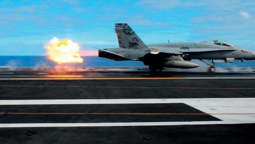
Figure 1.8: This fighter jet is accelerating.
t v ∆ t 0 ∆ v ∆ t ∆ v SAMPLE Original material © Cambridge University Press & Assessment 2023. This material is not final and is subject to further changes prior to publication. Any references or material related to answers, grades, papers or examinations are based on the opinion of the author(s)
Consider the graph of velocity against time in Figure 1.9. Imagine approximating the straight line with a staircase. The area under the staircase is the change in position since at each step the velocity is constant. If we make the steps of the staircase smaller and smaller, the area under the line and the area under the staircase will be indistinguishable and so we have the general result that:
KEY POINT
The area under the curve in a velocity against time graph is the change in position; in other words, the displacement.
From Figure 1.9 this area is (the shape is a trapezoid):
We get a final formula if we combine s = si + ut + 1 2 at 2 with v = u + at
From the second equation, we find t = v u a .
Substituting in the first equation we get:
This becomes:
Usually si = 0 so this last equation is usually written as v
2as
This formula is useful to solve problems in which no information about time is available.
In summary, for motion along a straight line with constant acceleration:
But v = u + at, so this becomes:
Δs = ( u + u + at 2 )t = ut + 1 2 at 2
So we have two for mulas for position in the case of uniformly accelerated motion (recall that Δs = s si ):
s = si + ( u + v 2 )t or Δs = ( u + v 2 )t
s = si + ut + 1 2 at 2 or Δs = ut + 1 2 at 2
Graphs of position against time for uniformly accelerated motion are parabolas (Figure 1.10). If the parabola ‘holds water’ (concave up) the acceleration is positive. If its concave down, the acceleration is negative.
1 Kinematics 19
s si = u v u a + 1 2 a ( v u a ) 2 = uv a u 2 a + 1 2 v 2 a uv a + 1 2 u 2 a = v 2 u 2 2a
v 2 = u 2 + 2a(s si) or v 2 = u 2 + 2aΔs
2 = u 2
+
v = u + at Δs = ( u + v 2 )t Δs = ut + 1 2 at 2 v 2 = u 2 + 2aΔs
Figure 1.10: Graphs of position s against time t for uniformly accelerated motion. a Positive acceleration. b Negative acceleration.
Δs = ( u + v 2 )t
Figure 1.9: The straight-line graph may be approximated by a staircase.
Time Velocity v u t 0 t 0 0 t s s ab SAMPLE Original material © Cambridge University Press & Assessment 2023. This material is not final and is subject to further changes prior to publication. Any references or material related to answers, grades, papers or examinations are based on the opinion of the author(s)
EXAM TIP
Table 1.2 summarises the meaning of the gradient and area for the different motion graphs.
Graph of …GradientArea position against time velocity velocity against time accelerationchange in position, i.e. displacement acceleration against time change in velocity
Table 1.2: Information that can be derived from motion graphs
The equations of kinematics can be used only for motion on a straight line with constant acceleration. (If the initial position is zero, Δs may be replaced by just s.)
CHECK YOURSELF 2
The graph in Figure 1.11 shows the variation of position with time.
WORKED EXAMPLE 1.3
A particle has an initial velocity 2.00 m s−1 Its acceleration is a = 4.00 m s−2. Find its displacement after 10.0 s.
Answer
Displacement is the change of position, i.e. Δs = s si. We use the equation:
Δs = ut + 1 2 at 2
= 2.00 × 10.0 + 1/2 × 4.00 × 10. 0 2
= 220 m
WORKED EXAMPLE 1.4
A car has an initial velocity of u = 5.0 m s−1 After a displacement of 20 m, its velocity becomes 7.0 m s−1. Find the acceleration of the car.
Answer
Here, Δs = s si = 20 m.
So, use v2 = u2 + 2aΔs to find a.
7.02 = 5.02 + 2a × 20
24 = 40a
Therefore, a = 0.60 m s−2
WORKED EXAMPLE 1.5
A body has an initial velocity of 4.0 m s−1. After 6.0 s the velocity is 12 m s−1. Determine the displacement of the body in the 6.0 s.
Answer
We know u, v and t. We can use: Δ
Δs = 48 m
20 PHYSICS FOR THE IB DIPLOMA: COURSEBOOK
( v + u 2 )t to
4.0 2
s =
get: Δs = ( 12 +
) × 6.0
a positive b negative c zero. 0 t /s s /m 0.5 0.5 1.0 1.0 1.5 2.5 0.5 1.0 2.0
Indicate the intervals of times for which the acceleration is:
SAMPLE Original material © Cambridge University Press & Assessment 2023. This material is not final and is subject to further changes prior to publication. Any references or material related to answers, grades, papers or examinations are based on the opinion of the author(s)
Figure 1.11
CONTINUED
A slower method would be to use v = u + at to find the acceleration:
12 = 4.0 + 6.0a
⇒ a = 1.333 m s −2
Then use the value of a to find Δs:
Δs = ut + 1 2 at 2 = 4.0 × 6.0 + 1 2 × 1.333 × 36 = 48 m
WORKED EXAMPLE 1.6
A ball, X, starts moving to the right from rest with a constant acceleration of 2.0 m s−2 2.0 s later, a second ball, Y, starts moving to the right with a constant velocity of 9.0 m s−1. Both balls start from the same position.
Determine the position of the balls when they meet. Describe what is going on.
Answer
Let the two balls meet t s after X starts moving.
The position of X is:
sX = 1 2 at 2 = 1 2 × 2.0 × t 2 = t 2
The position of Y is:
sY = 9(t − 2)
(The factor t – 2 must be considered because, after t s, Y has actually been moving for only t 2 seconds.)
These two positions are equal when the two balls meet, and so:
t 2 = 9(t 2)
Solving the quadratic equation we find t = 3.0 s and 6.0 s. At these times the positions are 9.0 m and 36 m. At 3.0 s Y caught up with X and passed it. At 6.0 s X caught up with Y and passed it. (Making position–time graphs here is instructive.)
1 Kinematics 21
SAMPLE Original material © Cambridge University Press & Assessment 2023. This material is not final and is subject to further changes prior to publication. Any references or material related to answers, grades, papers or examinations are based on the opinion of the author(s)
WORKED EXAMPLE 1.7
A particle starts out from the origin with velocity 10 m s−1 and continues moving at this velocity for 5 s. The velocity is then abruptly reversed to 5 m s−1 and the object moves at this velocity for 10 s.
For this motion find:
a the change in position, i.e. the displacement
b the total distance travelled
c the average speed
d the average velocity
Answer
The problem is best solved using the velocity–time graph, which is shown in Figure 1.12.
a The initial position is zero. So, after 5.0 s, the position is 10 × 5.0 m = 50 m (the area under the first part of the graph). In the next 10 s, the displacement changes by 5.0 × 10 = 50 m (the area under the second part of the graph). So the change in position (the displacement) = 50 50 = 0 m.
b Take the initial velocity as moving to the right. The object moved towards the right, stopped and returned to its starting position. (We know this because the displacement was 0.) The distance travelled is 50 m moving to the right and 50 m coming back, giving a total distance travelled of 100 m.
c The average speed is 100 15 = 6.7 m s −1
d The average velocity is z ero, since the displacement is zero.
22 PHYSICS FOR THE IB DIPLOMA: COURSEBOOK
Figure 1.12
1015 t 0/s –5 –10 5 10 v /ms–1 5 SAMPLE Original material © Cambridge University Press & Assessment 2023. This material is not final and is subject to further changes prior to publication. Any references or material related to answers, grades, papers or examinations are based on the opinion of the author(s)
WORKED EXAMPLE 1.8
An object with an initial velocity 20 m s−1 and initial position of 75 m experiences a constant acceleration of 2 m s−2. Sketch the position–time graph for this motion for the first 20 s.
Answer
Use the equation s = si + ut + 1 2 at 2. Substituting the values we know, the position is given by s = 75 + 20t t2. This is the function we must graph. The result is shown in Figure 1.13.
WORKED EXAMPLE 1.9
An object is thrown vertically upwards with an initial velocity of 20 m s−1 from the edge of a cliff that is 25 m from the sea below, as shown in Figure 1.14. Determine:
a the ball’s maximum height
b the time taken for the ball to reach its maximum height
c the time to hit the sea
d the speed with which it hits the sea (You may approximate g to 10 m s−2.)
At 5 s the object reaches the origin and overshoots it. It returns to the origin 10 s later (t = 15 s). The furthest it gets from the origin is 25 m. The velocity at 5 s is 10 m s−1 and at 15 s it is 10 m s−1. At 10 s the velocity is zero.
A special acceleration
Assuming that we can neglect air resistance and other frictional forces, an object thrown into the air will experience the acceleration of free fall while in the air. This is an acceleration caused by the attraction between the earth and the body. The magnitude of this acceleration is denoted by g. Near the surface of the earth g = 9.8 m s−2. The direction of this acceleration is always vertically downwards. (We will sometimes approximate g to 10 m s−2.)
Answer
We have motion on a vertical line so we will use the symbol y for position (Figure 1.15a). We take the direction up to be positive. The zero for position is the ball’s initial position.
1 Kinematics 23
Figure 1.13
Figure 1.14: A ball is thrown upwards from the edge of a cliff.
20ms–1 25m –80 –60 5101520 t 0/s –20 –40 20 40 s /m SAMPLE Original material © Cambridge University Press & Assessment 2023. This material is not final and is subject to further changes prior to publication. Any references or material related to answers, grades, papers or examinations are based on the opinion of the author(s)
a Displacement upwards is positive. b The highest point is the zero of position. Here we take displacement downwards to be positive.
a The quickest way to get the answer to this part is to use v2 = u2 2gy. (The acceleration is a = g.)
At the highest point v = 0, and so:
0 = 20 2 2 × 10y
⇒ y = 20 m
b At the highest point the object’s velocity is zero. Using v = 0 in v = u gt gives:
0 = 20 10 × t
t = 20 10 = 2.0 s
c There are many ways to do this. One is to use the displacement arrow shown in blue in Figure 1.15a. Then, when the ball hits the sea, y = 25 m. Now use the formula y = ut 1 2 gt 2 to find an equation that only has the variable t:
− 25 = 20 × t 5 × t 2
t 2 4t 5 = 0
This is a quadratic equation. Using your calculator you can find the two roots as 1.0 s and 5.0 s. Choose the positive root to find the answer
t = 5.0 s.
Another way of looking at this is shown in Figure 1.15b. Here we start at the highest point and take the direction down to be positive. Then, at the top y = 0, at the sea y = +45 m and a = +10 m s−2. Now, the initial velocity is zero because we take our initial point to be at the top.
Using y = ut + 1 2 gt 2 with u = 0, we find:
45 = 5 t 2
⇒ t = 3.0 s
This is the time to fall to the sea. It took 2.0 s to reach the highest point, so the total time from launch to hitting the sea is:
2.0 + 3.0 = 5.0 s.
d Use v = u gt and t = 5.0 s to get v = 20 10 × 5.0 = 30 m s−1. The speed is then 30 m s−1
(If you prefer the diagram in Figure 1.15b for working out part c and you want to continue this method for part d, then you would write v = u + gt with t = 3.0 s and u = 0 to get v = 10 × 3.0 = +30 m s−1.)
CHECK YOURSELF 3
A ball is thrown vertically upwards with a speed of 20 m s−1 and another vertically downwards with the same speed and from the same height. What interval separates the landing times of the two balls? (Take g = 10 m s−2.)
24 PHYSICS FOR THE IB DIPLOMA: COURSEBOOK
Figure 1.15: Diagrams for solving the ball’s motion.
CONTINUED 20ms–1 a b 0 y /m 45m y /m –25m 0
CONTINUED SAMPLE Original material © Cambridge University Press & Assessment 2023. This material is not final and is subject to further changes prior to publication. Any references or material related to answers, grades, papers or examinations are based on the opinion of the author(s)
TEST YOUR UNDERSTANDING
5 The initial velocity of a car moving on a straight road is 2.0 m s−1. It becomes 8.0 m s−1 after travelling for 2.0 s under constant acceleration. Find the acceleration.
6 A car accelerates from rest to 28 m s−1 in 9.0 s. Find the distance it travels.
7 A particle has an initial velocity of 12 m s−1 and is brought to rest over a distance of 45 m. Find the acceleration of the particle.
8 A particle at the origin has an initial velocity of −6.0 m s−1 and moves with an acceleration of 2.0 m s−2. Determine when its position will become 16 m.
9 A plane starting from rest takes 15.0 s to take off after speeding over a distance of 450 m on the runway with constant acceleration. Find the take-off velocity.
10 A particle starts from rest with constant acceleration. After travelling a distance d the speed is v. What was the speed when the particle had travelled a distance d 2 ?
11 A car is travelling at 40.0 m s−1. The driver sees an emergency ahead and 0.50 s later slams on the brakes. The deceleration of the car is 4.0 m s−2.
a Find the distance travelled before the car stops.
b Calculate the stopping distance if the driver could apply the brakes instantaneously without a reaction time.
c Calculate the difference in your answers to a and b.
d Assume now that the car was travelling at 30.0 m s−1 instead. Without performing any calculations, state whether the answer to c would now be less than, equal to or larger than before. Explain your answer.
12 Two balls are dropped from rest from the same height. One of the balls is dropped 1.00 s after the other. Air resistance is ignored.
a Find the distance that separates the two balls 2.00 s after the second ball is dropped.
b Explain what happens to the distance separating the balls as time goes on.
13 A particle moves in a straight line with an acceleration that varies with time as shown in Figure 1.16. Initially the velocity of the object is 2.00 m s−1
a Find the maximum velocity reached in the first 6.00 s of this motion.
b Draw a graph of the velocity against time.
14 The graph in Figure 1.17 shows the variation of velocity with time of an object. Find the acceleration at 2.0 s.
1 Kinematics 25
Figure 1.16
0 0246 3 9 6 t /s a /ms–2 4 0 2 4 6 8 0123 t /s v /ms–1 SAMPLE Original material © Cambridge University Press & Assessment 2023. This material is not final and is subject to further changes prior to publication. Any references or material related to answers, grades, papers or examinations are based on the opinion of the author(s)
Figure 1.17
CONTINUED
15 Your brand-new convertible is parked 15 m from its garage when it begins to rain. You do not have time to get the keys, so you begin to push the car towards the garage. The maximum acceleration you can give the car is 2.0 m s−2 by pushing and 3.0 m s−2 by pulling back on the car. Find the least time it takes to put the car in the garage. (Assume that the car and the garage are point objects.)
16 A stone is thrown vertically up from the edge of a cliff 35.0 m from the sea (Figure 1.18). The initial velocity of the stone is 8.00 m s−1
v
c the velocity just before hitting the sea
d the distance the stone covers
e the average speed and the average velocity for this motion
17 A ball is thrown upwards from the edge of a cliff with velocity 20.0 m s−1. It reaches the bottom of the cliff 6.0 s later. Take g = 10 m s−2.
a Determine the height of the cliff.
b Calculate the speed of the ball as it hits the ground.
18 A toy rocket is launched vertically upwards with acceleration 3.0 m s−2. The fuel runs out when the rocket reaches a height of 85 m.
a Calculate the velocity of the rocket when the fuel runs out.
b Determine the maximum height reached by the rocket.
c Draw a graph to show the variation of
i the velocity of the rocket
ii the position of the rocket from launch until it reaches its maximum height
Determine:
a the maximum height of the stone
b the time when it hits the sea
1.3 Graphs of motion
If the acceleration is constant the equations derived in Section 1.2 hold and we can use them to analyse a motion problem. But if acceleration is not constant
SAMPLE Original material © Cambridge University Press & Assessment 2023. This material is not final and is subject to further changes prior to publication. Any references or material related to answers, grades, papers or examinations are based on the opinion of the author(s)
26 PHYSICS FOR THE IB DIPLOMA: COURSEBOOK
Figure 1.18
d Calculate the time the rocket takes to fall to the ground from its maximum height. =8.00ms–1 35.0m
these equations do not apply and cannot be used. But we can still analyse a motion using graphs. Our main tools will be those provided in Table 1.1.
Consider the graph of position against time shown in Figure 1.19.
Working in exactly the same way we can find the shape of the acceleration-against-time graph by examining the gradient of the velocity graph we just obtained. The result is Figure 1.21.
We would like to predict the shape of the graph of velocity against time. We use the fact that velocity is the gradient of the position-against-time graph. We see that at t = 0 the gradient is positive. As time increases the gradient is still positive but gets smaller and smaller and at t = 0.25 s it becomes zero. It then becomes negative. It gets more and more negative, reaching its most negative value at t = 0.5 s. It remains negative past 0.5 s but the curve gets less steep and the gradient becomes zero again at 0.75 s. From then it becomes positive and increases until 1.0 s. These observations lead us to the velocity-against-time graph shown in Figure 1.20. Note that it is the shape we are after, not detailed numerical values of velocity; hence there is no need to put numbers on the vertical axis.
Look at the motion in Figure 1.22.
a State the time(s) at which the acceleration is zero.
b State the time(s) at which the acceleration is negative.
c At what time is the acceleration most negative?
d At 2.3 s, do you expect the displacement to be positive or negative and why?
1 Kinematics 27
Figure 1.21: Acceleration graph corresponding to the velocity graph of Figure 1.20.
CHECK YOURSELF 4
0 t / s velocity 0.2 0.2 0.4 0.4 0.6 0.8 1.0 1.5 2.5 0.5 1.0 2.0
t /s a 0.2 0.4 0.6 0.8 1.0 t /s 0.2 0.4 0.6 0.8 1.0 v
Figure 1.22
Figure 1.19: Position against time for accelerated motion.
0 t /s s /m 0.5 0.5 1.0 1.0 0.2 0.4 0.6 0.8 1.0 SAMPLE Original material © Cambridge University Press & Assessment 2023. This material is not final and is subject to further changes prior to publication. Any references or material related to answers, grades, papers or examinations are based on the opinion of the author(s)
Figure 1.20: The velocity graph corresponding to the graph of Figure 1.19.
TEST YOUR UNDERSTANDING
19 The graph in Figure 1.23 shows the variation of the position of a moving object with time. Draw the graph showing the variation of the velocity of the object with time.
21 The graph in Figure 1.25 shows the variation of the position of a moving object with time. Draw the graph showing the variation of the velocity of the object with time.
20 The graph in Figure 1.24 shows the variation of the position of a moving object with time. Draw the graph showing the variation of the velocity of the object with time.
22 The graph in Figure 1.26 shows the variation of the velocity of a moving object with time. Draw the graph showing the variation of the position of the object with time. The initial position is zero.
28 PHYSICS FOR THE IB DIPLOMA: COURSEBOOK
Figure 1.23
Figure 1.24
Figure 1.25
0.50 t /s 11.522.53 s 0123456 t /s 7 s 0.5 011.52 t /s s 0.5 011.52 t /s v SAMPLE Original material © Cambridge University Press & Assessment 2023. This material is not final and is subject to further changes prior to publication. Any references or material related to answers, grades, papers or examinations are based on the opinion of the author(s)
Figure 1.26
CONTINUED
23 The graph in Figure 1.27 shows the variation of the velocity of a moving object with time. Draw the graph showing the variation of the position of the object with time (assuming the initial position to be zero).
Draw a graph to show how velocity varies with time. The initial velocity is zero.
26 The graph in Figure 1.30 shows how acceleration varies with time.
24 The graph in Figure 1.28 shows the variation of the velocity of a moving object with time. Draw the graph showing the variation of the acceleration of the object with time.
Draw a graph to show how velocity varies with time. The initial velocity is zero.
27 The graph in Figure 1.31 shows the position against time of an object moving in a straight line. Four points on this graph have been selected.
25 The graph in Figure 1.29 shows how acceleration varies with time.
a Is the velocity between A and B positive, zero or negative?
b What can you say about the velocity between B and C?
c Is the acceleration between A and B positive, zero or negative?
d Is the acceleration between C and D positive, zero or negative?
1 Kinematics 29
Figure 1.27
Figure 1.28
Figure 1.29
Figure 1.30
Figure 1.31
1 0234 t /s v 0.5 011.52 t /s v Time Acceleration Time Acceleration A BC D x t 0 SAMPLE Original material © Cambridge University Press & Assessment 2023. This material is not final and is subject to further changes prior to publication. Any references or material related to answers, grades, papers or examinations are based on the opinion of the author(s)
28 Sketch velocity–time plots (no numbers are necessary on the axes) for the following motions.
a A ball is dropped from a certain height and bounces off a hard floor. The speed just before each impact with the floor is the same as the speed just after impact. Assume that the time of contact with the floor is negligibly small.
1.4 Projectile motion
Figure 1.32 shows the positions of two objects every 0.2 s: the first was simply allowed to drop vertically from rest; the other was launched horizontally with no vertical component of velocity. We see that in the vertical direction, both objects fall the same distance in the same time and so will hit the ground at the same time.
b A cart slides with negligible friction along a horizontal air track. When the cart hits the ends of the air track it reverses direction with the same speed it had right before impact. Assume the time of contact of the cart and the ends of the air track are negligibly small.
c A person jumps from a hovering helicopter. After a few seconds she opens a parachute. Eventually she will reach a terminal speed and will then land.
THEORY OF KNOWLEDGE
How do we understand this fact? Consider Figure 1.33, in which a black ball is projected horizontally with velocity v. A blue ball is allowed to drop vertically from the same height.
Figure 1.33a shows the situation when the balls are released as seen by an observer X at rest on the ground. But suppose there is an observer Y, who moves to the right with velocity v 2 with respect to the ground. What does Y see? Observer Y sees the black ball moving to the right with velocity v 2 and the blue ball approaching with velocity − v 2 Figure 1.18b). The motions of the two balls are therefore identical (except for direction). So this observer will determine that the two bodies reach the ground at the same time. Since time is absolute in Newtonian physics, the two bodies must reach the ground at the same time as far as any other observer is concerned as well.
30 PHYSICS FOR THE IB DIPLOMA: COURSEBOOK
y /m x /m 020406080100 –5 –4 –3 –2 –1 0 CONTINUED
Figure 1.32: A body dropped from rest and one launched horizontally cover the same vertical distance in the same time.
SAMPLE Original material © Cambridge University Press & Assessment 2023. This material is not final and is subject to further changes prior to publication. Any references or material related to answers, grades, papers or examinations are based on the opinion of the author(s)
Figure 1.33: a A ball projected horizontally and one simply dropped from rest from the point of view of observer X. Observer Y is moving to the right with velocity v 2 with respect to the ground.
b From the point of view of observer Y, the black and the blue balls have identical motions.
The motion of a ball that is projected at some angle can be analysed by separately looking at the horizontal and the vertical directions. All we have to do is consider two motions, one in the horizontal direction in which there is no acceleration and another in the vertical direction in which we have an acceleration, g
Consider Figure 1.34, where a projectile is launched at an angle θ to the horizontal with speed u
The components of the initial velocity vector are
u x = u cos θ and u y = u sin θ
At some later time t the components of velocity are v x and v y . In the x-direction there is zero acceleration and in the y-direction, the acceleration is g and so:
Horizontal directionVertical direction
The green vector in Figure 1.35a shows the position of the projectile t seconds after launch. The red arrows in Figure 1.35b show the velocity vectors and their components. Here the true vector nature of what we have been calling position comes into its own.
The position of the projectile is determined by the position vector → r , a vector from the origin to the position of the projectile. The components of this vector are x and y
Figure 1.35: a The position of the particle is determined if we know the x- and y-components of the position vector. b The velocity vectors for projectile motion are tangents to the parabolic path.
EXAM TIP
All that we are doing is using the formulas from the previous section for velocity and position –v = u + at and s = ut + 1 2 at 2 – and rewriting them separately for each direction x and y. In the x-direction there is zero acceleration, and in the y-direction there is an acceleration –g
We would like to know the x- and y-components of the position vector. We now use the formula for position. In the x-direction:
x = u x t and so x = ut cos θ
In the y-direction:y = u y t 1 2 gt 2 and so y = ut sin θ 1 2 gt 2
1 Kinematics 31
v x = u cos θ v y = u sin θ − gt
θ u ux uy 0.51.0 a 1.52.0 x 0/m –5 5 10 15 20 y /m x y P 0.51.0 b 1.52.0 x 0/m –5 5 10 15 20 y /m
Figure 1.34: A projectile is launched at an angle θ to the horizontal with speed u
CONTINUED
XY ab XY –v v 2 v 2 –v 2 v 2 SAMPLE Original material © Cambridge University Press & Assessment 2023. This material is not final and is subject to further changes prior to publication. Any references or material related to answers, grades, papers or examinations are based on the opinion of the author(s)
In summary:
Horizontal directionVertical direction
v x = u cos θ v y = u sin θ gt
x = ut cos θ y = ut sin θ 1 2 gt 2
The equation with ‘squares of speeds’ is a bit trickier (carefully review the following steps). It is:
v2 = u2 2gy
Since v2 = v x 2 + v y 2 and u2 = u x 2 + u y2, and in addition
v x 2 = u x2, this is also equivalent to:
v y 2 = u y 2 2gy
EXAM TIP
Always choose your x- and y-axes so that the origin is the point where the launch takes place.
CHECK YOURSELF 5
A projectile is launched with kinetic energy K at 60° to the horizontal. What is the kinetic energy of the projectile at the highest point of its path?
(Kinetic energy is equal to 1 2 mv 2.)
WORKED EXAMPLE 1.10
A body is launched with a speed of 18.0 m s−1 at the following angles:
a 30° to the horizontal
b 0° to the horizontal
c 90° to the horizontal
Find the x- and y-components of the initial velocity in each case.
Answer
a v x = u cos θ v y = u sin θ
v x = 18.0 × cos 30° v y = 18.0 × sin 30°
v x = 15.6 m s−1 v y = 9.00 m s−1
b v x = 18.0 m s−1 v y = 0 m s−1
c v x = 0 v y = 18.0 m s−1
WORKED EXAMPLE 1.11
For a projectile launched at some angle above the horizontal, sketch graphs to show the variation with time of:
a the horizontal component of velocity
b the vertical component of velocity
Answer
The graphs are shown in Figure 1.36.
WORKED EXAMPLE 1.12
An object is launched horizontally from a height of 20 m above the ground with speed 15 m s−1. Determine:
a the time at which it will hit the ground
b the horizontal distance travelled
c the speed with which it hits the ground
(Take g = 10 m s−2.)
Answer
a The launch is horizontal, i.e. θ = 0°, and so the formula for vertical position is just y = 1 2 gt 2 The object will hit the ground when y = 20 m.
32 PHYSICS FOR THE IB DIPLOMA: COURSEBOOK
Time vx 0 Time 0 vy
Figure 1.36: Answer to worked example 1.11
SAMPLE Original material © Cambridge University Press & Assessment 2023. This material is not final and is subject to further changes prior to publication. Any references or material related to answers, grades,
or
are based on the opinion of the author(s)
papers
examinations
CONTINUED
Substituting the values, we find:
− 20 = − 5t 2
⇒ t = 2.0s
b The horizontal position is found from x = ut Substituting values:
x = 15 × 2.0 = 30 m (Remember that θ = 0°.)
c Use v2 = u2 2gy to get:
v2 = 152 2 × 10 × ( 20)
v = 25 m s−1
WORKED EXAMPLE 1.13
An object is launched horizontally with a velocity of 12 m s−1. Determine:

a the vertical component of velocity after 4.0 s
b the x- and y-components of the position vector of the object after 4.0 s.
Answer
a The launch is again horizontal, i.e. θ = 0°, so substitute this value in the formulas. The horizontal component of velocity is 12 m s−1 at all times.
From v y = gt, the vertical component after 4.0 s is v y = 40 m s−1.
b The coordinates after time t are:
x = ut y = − 1 2 gt 2
x = 12 . 0 × 4 . 0 y = − 5 × 16
x = 48 m and y = − 80 m
At what point in time does the vertical velocity component become zero? Setting v y = 0 we find:
0 = u sin θ gt
⇒ t = u sin θ g
1 Kinematics 33
Figure 1.37 shows an object thrown at an angle of θ = 30° to the horizontal with initial speed 20 m s−1. The position of the object is shown every 0.2 s. Note how the dots get closer together as the object rises (the speed is decreasing) and how they move apart on the way down (the speed is increasing). It reaches a maximum height of 5.1 m and travels a horizontal distance of 35 m. The photo in Figure 1.38 shows an example of projectile motion.
Figure 1.37: A launch at of θ = 30° to the horizontal with initial speed 20 m s−1
Figure 1.38: A real example of projectile motion.
EXAM TIP
0 1 2 3 4 5 05101520253035 x/m y /m x u0 y
Worked example 1.13 is a basic problem— you must know how to do this!
SAMPLE Original material © Cambridge University Press & Assessment 2023. This material is not final and is subject to further changes prior to publication. Any references or material related to answers, grades, papers or examinations are based on the opinion of the author(s)
The time when the vertical velocity becomes zero is, of course, the time when the object attains its maximum height. What is this height? Going back to the equation for the vertical component of position, we find that when:
t = u sin θ g
y is given by:
ymax = u u sin θ g sin θ − 1 2 g ( u sin θ g )2
ymax = u 2 sin 2 θ 2g
What about the maximum displacement in the horizontal direction (called the range)? At this point y is zero. We can find the time by setting y = 0 in the formula for y but it is easier to notice that since the path is symmetrical the time to cover the range is double the time to get to the top, so t = 2u sin θ g
EXAM TIP
You should not remember these formulas by heart. You should be able to derive them quickly.
Therefore the range is:
x = 2 u 2 sin θ cos θ g
A bit of trigonometry allows us to rewrite this as:
x = u 2 sin 2θ g
One of the identities in trigonometry is 2 sin θ cos θ = sin 2θ.
The maximum value of sin 2θ is 1, and this happens when 2θ = 90° (θ = 45°). In other words, we obtain the maximum range with a launch angle of 45°. This equation also says that there are two different angles of launch that give the same range for the same initial speed. These two angles add up to a right angle. (Can you see why?)
CHECK YOURSELF 6
On earth the maximum height and range of a projectile are H and R, respectively. The projectile is launched with the same velocity on a planet where the acceleration of free fall is 2g. What are the maximum height and range of the projectile on the planet?
WORKED EXAMPLE 1.14
A projectile is launched at 32.0° to the horizontal with initial speed 25.0 m s−1. Determine the maximum height reached. (Take g = 9.81 m s−2.)
Answer
The vertical velocity is given by v y = u sin θ gt and becomes zero at the highest point. Thus:
t = u sin θ g
t = 25.0 × sin 32.0° 9.81
t = 1.35 s
Substituting in the formula for y, y = ut sin θ 1 2 gt 2 , we get:
y = 25 × sin 32.0° × 1.35 − 1 2 × 9.81 × 1.35 2
y = 8.95 m
Equivalently, 0 = (u sin θ) 2 − 2gy ⇒
y = (25.0 × sin 32.0°) 2 2 × 9.81 = 8.95 m
WORKED EXAMPLE 1.15
A projectile is launched horizontally from a height of 42 m above the ground. As it hits the ground, the velocity makes an angle of 55° to the horizontal. Find the initial velocity of launch. (Take g = 9.8 m s−2.)
Answer
The time it takes to hit the ground is found from y = − 1 2 gt 2. (Here θ = 0° since the launch is horizontal.)
The ground is at y = 42 m and so: 42 = − 1 2 × 9.8 t 2
⇒ t = 2.928 s
Using v y = u sin θ gt, when the projectile hits the ground:
v y = 0 9.8 × 2.928
v y = 28.69 m s−1
34 PHYSICS FOR THE IB DIPLOMA: COURSEBOOK
Original material © Cambridge University Press & Assessment 2023. This material is not final and is subject to further changes prior to publication. Any references or material related to answers, grades, papers or examinations are based on the opinion of the author(s)
SAMPLE
CONTINUED
We know the angle the final velocity makes with the ground (Figure 1.39). Hence:
Links
In projectile motion we have a single constant force whose direction is always vertical. This force is the weight of the body. When the body is projected at an angle to the vertical the result is motion along a path that is parabolic. There is one other instance where again a force that is constant in magnitude and direction acts on a body. This is the case of motion of an electric charge in a uniform electric field. So we expect that a charge projected at an angle in a region of uniform electric field will also result in motion along a parabolic path and what we have learned in this chapter will apply to that case as well. See Chapter 19
Fluid resistance
The discussion of the previous sections has neglected air resistance forces. In general, whenever a body moves through a fluid (gas or liquid) it experiences a fluid resistance force that is directed opposite to the velocity. Typically F = kv for low speeds and F = kv2 for high speeds (where k is a constant). The magnitude of this force increases with increasing speed.
Imagine dropping a body of mass m from some height. Assume that the force of air resistance on this body is F = kv. Initially, the only force on the body is its weight,
which accelerates it downwards. As the speed increases, the force of air resistance also increases. Eventually, this force will become equal to the weight and so the acceleration will become zero: the body will then move at constant speed, called terminal speed, vT. This speed can be found from:
mg = kvT which leads to:
vT = mg k
Figure 1.40 shows how the speed and acceleration vary for motion with an air resistance force that is proportional to speed. The speed eventually becomes the terminal speed, and the acceleration becomes zero. The initial acceleration is g
Figure 1.40: a The variation with time of a speed. b Acceleration in motion with an air resistance force proportional to speed.
The effect of air resistance forces on projectiles is very pronounced. Figure 1.41 shows the positions of a projectile with (red) and without (blue) air resistance forces. With air resistance forces the range and maximum height are smaller and the shape is no longer symmetrical.
1 Kinematics 35
tan= vx vy vy vx θ θ 0 10 20 30 0510 a 1520 t /s v /ms–1 0 2 4 0510 b 1520 t /s a /ms–2 8 6 10
tan 55° = | v y v x | ⇒ v x = 28.69 tan 55° v x = 20.09 ≈ 20 m s −1
Figure 1.39
SAMPLE Original material © Cambridge University Press & Assessment 2023. This material is not final and is subject to further changes prior to publication. Any references or material related to answers, grades, papers or examinations are based on the opinion of the author(s)
The projectile hits the ground at a steeper angle.
WORKED EXAMPLE 1.16
The force of air resistance in the motion described by Figure 1.40 is given by F = 0.653v
Determine the mass of the projectile.
Answer
The terminal speed is 30 m s−1 and is given by
vT = mg k . Hence:
m = 0.653 × 30 9.8
m ≈ 2 . 0 kg
NATURE OF SCIENCE
The simple and the complex Careful observation of motion in the natural world led to the equations for motion with uniform acceleration along a straight line that we have used in this section. Thinking about what causes an object to move links to the idea of forces. However, although the material in this section is perhaps some of the ‘easiest’ material in your physics course, it does not enable you to understand the falling of a leaf off a tree. The falling leaf is complicated
TEST YOUR UNDERSTANDING
29 A ball rolls off a table with a horizontal speed of 2.0 m s−1. The table is 1.3 m high. Calculate how far from the table the ball will land.
30 Two particles are on the same vertical line. They are thrown horizontally with the same speed, 4.0 m s−1, from heights of 4.0 m and 8.0 m.
a Calculate the distance that will separate the two objects when both land on the ground.
b The particle at the 4.0 m height is now launched with horizontal speed u such that it lands at the same place as the particle launched from 8.0 m.
Calculate u.
because it is acted upon by several forces: its weight, but also air resistance forces that constantly vary as the orientation and speed of the leaf change. In addition, there is wind to consider as well as the fact that turbulence in air greatly affects the motion of the leaf. So the physics of the falling leaf is far away from the physics of motion along a straight line at constant acceleration. But learning the principles of physics in a simpler context allows its application in more involved situations.
31 For an object thrown at an angle of 40° to the horizontal at a speed of 20 m s−1, draw graphs of:
a horizontal velocity against time
b vertical velocity against time
c acceleration against time
32 Determine the maximum height reached by an object thrown with speed 24 m s−1 at 40° to the horizontal.
33 An object is thrown with speed 20.0 m s−1 at an angle of 50° to the horizontal. Draw graphs to show the variation with time of:
a the horizontal position
b the vertical position
36 PHYSICS FOR THE IB DIPLOMA: COURSEBOOK
0 500 1000 1500 0500100015002000250030003500 x /m y /m
Figure 1.41: The effect of air resistance on projectile motion.
SAMPLE Original material © Cambridge University Press & Assessment 2023. This material is not final and is subject to further changes prior to publication. Any references or material related to answers, grades, papers or examinations are based on the opinion of the author(s)
CONTINUED
34 A cruel man takes aim horizontally at a chimp that is hanging from the branch of a tree, as shown in Figure 1.42.
The chimp lets go of the branch as soon as the hunter pulls the trigger. Treating the chimp and the bullet as point particles, determine if the bullet will hit the chimp.
ii the angle to the horizontal the ball was launched at,
iii the acceleration of free fall on this planet.
b Make a copy of the graph and draw two arrows to represent the velocity and the acceleration vectors of the ball at t = 1.0 s.
c The ball is now launched under identical conditions from the surface of a different planet where the acceleration due to gravity is twice as large. Draw the path of the ball on your graph.
36 A stone is thrown with a speed of 20.0 m s−1 at an angle of 48° to the horizontal from the edge of a cliff 60.0 m above the surface of the sea.
a Calculate the velocity with which the stone hits the sea.
b Discuss qualitatively the effect of air resistance on your answer to a
35 A ball is launched from the surface of a planet. Air resistance and other frictional forces are neglected. The graph in Figure 1.43 shows the position of the ball every 0.20 s.
37 a State what is meant by terminal speed
b A ball is dropped from rest. The force of air resistance on the ball is proportional to the ball’s speed. Explain why the ball will reach terminal speed.
38 A projectile is launched with speed u at 45° to the horizontal. The projectile is at height h at two different times.
a Show that the horizontal distance separating those points is u g √ u 2 4gh
b Deduce, using the result in part a, the maximum height reached by this projectile.
39 A projectile is launched with some speed at some angle to the horizontal. At 1.0 s and at 5.0 s the height of the projectile from the ground is the same. What is the maximum height reached by this projectile?
(Take g = 10 m s–2.)
a Use this graph to determine:
i the components of the initial velocity of the ball,
1 Kinematics 37
Figure 1.42
Figure 1.43
0 2 4 6 8 10 0102030405060 x /m y /m SAMPLE Original material © Cambridge University Press & Assessment 2023. This material is not final and is subject to further changes prior to publication. Any references or material related to answers, grades, papers or examinations are based on the opinion of the author(s)
SELF-ASSESSMENT CHECKLIST
I am able to ...
define and distinguish between the concepts of position, displacement, average and instantaneous velocity and average and instantaneous acceleration 1.1 solve problems using the equations of kinematics
analyse motion through graphs
describe the effect of air resistance force on projectile motion
REFLECTION
move
Do you understand the difference between distance and displacement? Do you understand the difference between speed and velocity? Are you confident using the equations of kinematics? Do you know what information a graph of position versus time gives? Do you know what information a graph of velocity versus time gives? Can you explain why a body reaches terminal speed if it is acted upon by a speed dependent resistance force? Do you understand how to solve problems with projectile motion? Can you describe the effect of air resistance on the path of a projectile?
EXAM-STYLE QUESTIONS
You can find questions in the style of IB exams online in the digital coursebook.
CHECK YOURSELF ANSWERS
1 Let d be the distance between A and B and t1, t2 the travel times back and forth. Then
d = 15 t1 = 30 t2, i.e. t1 = 2 t2. The average speed is then v = 2d t1 + t2 = 2 × 30 t2 3 t2 = 20 m s −1
2 Positive for 1.0 s on, because curve is concave up, negative for 0 s to 1.0 s and zero at 1.0 s.
3 It takes 2 s to get to the maximum height and 2 to return so the required time is 4 s.
4 a Zero at about 0.4 s and 1.6 s.
b Negative from 0.4 s to 1.6 s.
c Most negative at 1.0 s.
d The displacement from 0 s to 1.0 s is about the same in magnitude as that from 1.0 s to 2.0 s so the displacement at 2.3 s will be positive.
5 K = 1 2 mu 2. At the highest point, KE = 1 2 mu 2 cos 2 60 ° = 1 2 mu 2 × 1 4 = K 4 .
6 Both H and R are inversely proportional to the acceleration of free fall and so both are halved.
38 PHYSICS FOR THE IB DIPLOMA: COURSEBOOK
Not yet Nearly there Ready to
1.3
1.4
1.4
Section
on
1.2
solve problems with projectile motion
SAMPLE Original material © Cambridge University Press & Assessment 2023. This material is not final and is subject to further changes prior to publication. Any references or material related to answers, grades, papers or examinations are based on the opinion of the author(s)


with IB teachers Digital Teacher’s Resource SAMPLE Original material © Cambridge University Press & Assessment 2023. This material is not final and is subject to further changes prior to publication. Any references or material related to answers, grades, papers or examinations are based on the opinion of the author(s)
Physics for the IB Diploma Together
Original material © Cambridge University Press & Assessment 2023. This material is not final and is subject to further changes prior to publication. Any references or material related to answers, grades, papers or examinations are based on the opinion of the author(s)
SAMPLE
41 1 PHYSICS FOR THE IB DIPLOMA: TEACHER’S RESOURCE Table of contents About the authors 00 How to use this series 00 How to use this Teacher’s Resource 00 About the Guide (syllabus) 00 About the assessment (examinations) 00 Integrating TOK in your Science lesson 00 A guide to academic writing 00 Teaching notes 00 Unit A Kinematics 00 1 Kinematics 00 1.1 Displacement, distance, speed and velocity 00 1.2 Uniformly accelerated motion: the equations of kinematics 00 1.3 Graphs of motion 00 1.4 Projectile motion 00 2 Forces and Newton’s laws 00 2.1 Forces and their direction 00 2.2 Newton’s laws of motion 00 2.3 Circular motion 00 3 Work, energy and power 00 3.1 Work 00 3.2 Conservation of mechanical energy 00 3.3 Power and efficiency 00 3.4 Energy transfers 00 4 Linear momentum 00 4.1 Newton’s second law in terms of momentum 00 4.2 Impulse and force–time graphs 00 4.3 Conservation of momentum 00 4.4 Kinetic energy and momentum 00 4.5 Two-dimensional collisions 00 SAMPLE Original material © Cambridge University Press & Assessment 2023. This material is not final and is subject to further changes prior to publication. Any references or material related to answers, grades, papers or examinations are based on the opinion of the author(s)
42 2
5 Rigid body mechanics 00 5.1 Kinematics of rotational motion 00 5.2 Rotational equilibrium and Newton’s second law 00 5.3 Angular momentum 00 6 Relativity 00 6.1 Reference frames and Lorentz transformations 00 6.2 Effects of relativity 00 6.3 Spacetime diagrams 00 Unit B The particulate nature of matter 00 7 Thermal energy transfers 00 7.1 Particles, temperature and energy 00 7.2 Specific heat capacity and change of phase 00 7.3 Thermal energy transfer 00 8 The greenhouse effect 00 8.1 Radiation from real bodies 00 8.2 Energy balance of the Earth 00 9 The gas laws 00 9.1 Moles, molar mass and the Avogadro constant 00 9.2 Ideal gases 00 9.3 The Boltzmann equation 00 10 Thermodynamics 00 10.1 Internal energy 00 10.2 The first law of thermodynamics 00 10.3 The second law of thermodynamics 00 10.4 Heat engines 11 Current and circuits 00 11.1 Potential difference, current and resistance 00 11.2 Voltage, power and emf 00 11.3 Resistors in electrical circuits 00 11.4 Terminal potential difference and the potential divider 00 Unit C Wave behaviour 00 12 Simple harmonic motion 00 12.1 Simple harmonic oscillations 00 12.2 Details of simple harmonic motion 00 12.3 Energy in simple harmonic motion 00 12.4 More about energy in SHM 00 SAMPLE Original material © Cambridge University Press & Assessment 2023. This material is not final and is subject to further changes prior to publication. Any references or material related to answers, grades, papers or examinations are based on the opinion of the author(s)
PHYSICS FOR THE IB DIPLOMA: TEACHER’S RESOURCE
43 3
13 The wave model 00 13.1 Mechanical pulses and waves 00 13.2 Transverse and longitudinal waves 00 13.3 Electromagnetic waves 00 13.4 Waves extension 00 14 Wave phenomena 00 14.1 Reflection and refraction 00 14.2 The principle of superposition 00 14.3 Diffraction and interference 00 14.4 Single-slit diffraction 00 14.5 Multiple slits 00 15 Standing waves and resonance 00 15.1 Standing waves 00 15.2 Standing waves on strings 00 15.3 Standing waves in pipes 00 15.4 Resonance and damping 00 16 The Doppler effect 00 16.1 The Doppler effect at low speeds 00 16.2 The Doppler effect for sound 00 Unit D Fields 00 17 Gravitation 00 17.1 Newton’s law of gravitation 00 17.2 Gravitational potential and energy 00 17.3 Motion in a gravitational field 00 18 Electric and magnetic fields 00 18.1 Electric charge, force and field 00 18.2 Magnetic field and force 00 18.3 Electrical potential and electrical potential energy 00 19 Motion in electric and magnetic fields 00 19.1 Motion in an electric field 00 19.2 Motion in a magnetic field 00 20 Electromagnetic induction 00 20.1 Electromagnetic induction 00 20.2 Generators and alternating current 00 Unit E Nuclear and quantum physics 00 21 Atomic physics 00 21.1 The structure of the atom 00 21.2 Quantization of angular momentum 00 SAMPLE Original material © Cambridge University Press & Assessment 2023. This material is not final and is subject to further changes prior to publication. Any references or material related to answers, grades, papers or examinations are based on the opinion of the author(s)
PHYSICS FOR THE IB DIPLOMA: TEACHER’S RESOURCE
The following items are available on Cambridge GO. For more information on how to access and use your digital resource, please see inside front cover.
44 4 PHYSICS
THE IB DIPLOMA: TEACHER’S RESOURCE 22 Quantum physics 00 22.1 Photons and the photoelectric effect 00 22.2 Matter waves 00 23 Nuclear physics 00 23.1 Mass defect and binding energy 00 23.2 Radioactivity 00 23.3 Nuclear properties and the radioactive decay law 00 24 Nuclear fission 00 24.1 Nuclear fission 00 25 Nuclear fusion and stars 00 25.1 Nuclear fusion 00 25.2 Stellar properties and the Hertzsprung–Russell diagram 00 25.3 Stellar evolution extension 00
resources
FOR
Digital
Worksheets 00 PowerPoints 00 End of chapter tests 00 Specimen papers 00 Coursebook answers 00 Workbook answers 00 Worksheet answers 00 End of chapter tests answers 00 Specimen paper answers (model answers) 00 Glossary 00 Acknowledgements 00 SAMPLE Original material © Cambridge University Press & Assessment 2023. This material is not final and is subject to further changes prior to publication. Any references or material related to answers, grades, papers or examinations are based on the opinion of the author(s)
How to use this Teacher’s Resource
This digital Teacher’s Resource contains both general guidance and teaching notes that help you deliver the content for the IB Physics course. You will find answers to the Coursebook and the Workbook questions on the supporting resources area of Cambridge GO—they are freely available to teachers only. There are teaching notes for each sub-chapter of the Coursebook. You can see an overview of where all topics are covered in the teaching plan in the ‘Resources’ column. Each set of teaching notes contains various features to help you deliver the topics covered in a unit/chapter.
At the start of each chapter is a teaching plan for the chapter. This summarises the topics covered in the chapter, including the number of learning hours recommended for each topic, an outline of the learning content, and the resources from this series that can be used to deliver the topic.
Teaching plan
This icon in the resources section indicates material that is available from Cambridge GO. Each chapter also includes information on any background knowledge that learners should have before studying content covered in the chapter.
BACKGROUND KNOWLEDGE
• Explain what an electromagnetic spectrum represents, the different types of radiations and their uses, the quantitative relationship between wavelength, frequency and energy of the radiations.
Syllabus overview
• At the start of each unit is a syllabus overview, which gives a brief outline of the content knowledge, practical skills and opportunities to cover assessment objectives covered in that section of the syllabus. It also provides links to related topic areas in other parts of the syllabus.
• The learning plan will enable you to identify the related learning intentions and success criteria from the coursebook chapter.
45 5 PHYSICS FOR THE IB DIPLOMA: TEACHER’S RESOURCE
number of learning hours Learning content Resources
Sub-chapterApproximate
SAMPLE Original material © Cambridge University Press & Assessment 2023. This material is not final and is subject to further changes prior to publication. Any references or material related to answers, grades, papers or examinations are based on the opinion of the author(s)
PHYSICS FOR THE IB DIPLOMA: TEACHER’S RESOURCE
LEARNING PLAN
Learning objectives
Success criteria
There is also a feature highlighting any common misconceptions associated with particular learning topics. Potential misunderstandings are identified, along with methods of eliciting evidence of these misconceptions from your class and suggestions on how to overcome them.
Misconception How to identify How to overcome
For each topic, there is a selection of lesson starter ideas, main teaching ideas and plenary ideas. You can pick out individual ideas that meet the needs of your class. The activities include suggestions for how they can be differentiated or used for assessment.
Differentiation ideas are provided for each topic, with ‘stretch and challenge’ activities, ideas to extend learning opportunities and ‘support’ activities, ideas and modifications for learners who need extra practice or help.
The cross-curricular links feature provides suggestions for linking to other areas of study within the Standard Level and Higher Level IB curriculum. Cross-topic links allow students to make connections between the different syllabus sections of the IB Physics course. They encourage students to approach Physics as a holistic topic and help them develop the skills required for approaching exam questions, which often drawn on several areas of the course.
This Teacher’s Resource includes a range of digital materials that you can download from Cambridge GO. (For more information about how to access and use your digital resource, please see inside front cover.)
You will find the glossary of terms for the Coursebook and Workbook and also answers to activities, worksheets and end of chapter tests within and at the end of this resource.
To help with lesson planning, a blank lesson plan template is available to download from Cambridge GO as part of this digital Teacher’s Resource.
More information about these approaches to learning and teaching is available to download from Cambridge GO as part of this digital Teacher’s Resource.
46 6
Original material © Cambridge University Press & Assessment 2023. This material is not final and is subject to further changes prior to publication. Any references or material related to answers, grades, papers or examinations are based on the opinion of the author(s)
SAMPLE
1 Kinematics
Teaching plan
Sub-chapterApproximate number of learning hours
1.1 Displacement, distance, speed and velocity
Learning content Resources
1
• Students learn the differences between displacement and distance and between velocity and speed.
Coursebook Section 1.1.
Test your understanding 1–4.
Exam-style questions
Workbook
Exercise 1.1
Teacher’s resource
1.2 Uniformly accelerated motion: the equations of kinematics
2
• Students learn to use the equations of motion.
Coursebook Section 1.2.
Test your understanding 5–18.
Exam-style questions
Workbook
Exercise 1.2
Teacher’s resource
1.3 Graphs of motion
2
• Students learn to sketch and interpret displacement–time and velocity–time graphs
Coursebook Section 1.3.
Test your understanding 19–28.
Exam-style questions
Workbook
Exercise 1.2
Teacher’s resource
1.4 Projectile motion
2
• Students learn to apply the equations of motion in the horizontal and vertical directions
• Students consider the effects of fluid resistance on projectile motion
Coursebook Section 1.4.
Test your understanding 29–39.
Exam-style questions
Workbook
SAMPLE Any references or material related to answers, grades, papers or examinations are based on the opinion of the author(s)
Exercise 1.4
47 2
PHYSICS FOR THE IB DIPLOMA: TEACHER’S RESOURCE
Physics for the IB Diploma – Bonsall © Cambridge University Press 2023
Teacher’s resource Original material © Cambridge University Press & Assessment 2023. This material is not final and is subject to further changes prior to publication.
BACKGROUND KNOWLEDGE
• Students should be familiar with the units for distance (m), time (s), speed (m/s) and acceleration (m/s2), although they may not have seen negative indices in units, such as in m s–1 and m s–2
• Students may have already have used the equation linking average speed, distance and time taken, and also the equation linking acceleration, change in speed and time taken.
Syllabus overview
• Some students may have seen speed–time or distance–time graphs.
• Students should be able to rearrange equations that contain addition/subtraction, multiplication/division and square/square root functions.
• Students should be able to sketch and interpret graphs that are straight lines or curves and be familiar with the meaning of gradient.
• This chapter covers the equations of motion in a straight line under zero or uniform acceleration and distinguishes between scalar and vector quantities in the context of motion.
• Students also get practice in sketching and interpreting graphs showing the variation of displacement with time, velocity with time and acceleration with time.
• The calculations of projectile motion are included, and students qualitatively describe the effects of fluid resistance on motion.
1.1 Displacement, distance, speed and velocity
LEARNING PLAN
Learning objectives
• Learn the difference between displacement and distance.
• Learn the difference between speed and velocity.
Common misconceptions
Misconception
Velocity is just a more scientific word for speed and means the same thing.
Students may use the symbol s to mean speed.
Success criteria
• Students should be able to describe the meaning of each term correctly.
• Students should be able to give a definition, in words or as an equation, for each term.
How to identify
After students learn about scalars and vectors and the meanings of speed and velocity, ask for a definition of each.
The symbol s will be used incorrectly.
How to overcome
Students can remember which quantity is scalar and which is vector by their initial letters.
v stands for velocity and vector;
s stands for speed and scalar.
Not all symbols are derived from English language words. The origin of s comes from the Latin word spatium (pronounced ‘space-ium’) meaning the distance between two locations.
48 3 PHYSICS FOR THE IB DIPLOMA: TEACHER’S RESOURCE Physics for the IB Diploma – Bonsall © Cambridge University Press 2023
SAMPLE Original material © Cambridge University Press & Assessment 2023. This material is not final and is subject to further changes prior to publication. Any references or material related to answers, grades, papers or examinations are based on the opinion of the author(s)
PHYSICS FOR THE IB DIPLOMA: TEACHER’S RESOURCE
Starter ideas
1 How far have you gone? (2 minutes)
Resources: n/a
Description and purpose: Ask students to sit in the same positions as they did in the previous lesson that was held in the same room. Now ask them to discuss with a learning partner how far they have travelled since the previous lesson. The answer could be several kilometres, for example, around the school, to home and back, and so on. Alternatively, the answer could be no distance, because they have ended up in the same place as last time. Use the idea to introduce the difference between distance and displacement.
2 How fast? (10 minutes)
Resources: A number of photographs, pictures or videos from the internet of animals, runners, cars, aeroplanes, the Earth moving round the sun and so on.
Description and purpose: Ask students to place the objects in the pictures in order from slowest to fastest. In groups, students can suggest values for the top speed of each object. Groups can then compare their results. As students discuss results, it should become clear that speeds can be measured in different units. Write some typical results on the board so that students can self-assess their estimates. Ask: Do you understand the different units that you use?
Challenge students to come up with as many different units for speed as they can. Ask: What units might an astronomer use to measure the speed of a galaxy moving away from us?
Main teaching ideas
1 Using the equation for average speed (20 minutes)
Resources: Calculators, Coursebook Test Your Understanding questions
Description and purpose: Briefly explain the equation for speed. Point out that average speed is calculated from total distance total time
Introduce the SI system of units. Explain the need for an international system. Ensure that all students can rearrange this equation successfully. Do they understand how to convert between different units of distance, such as millimetres, centimetres and kilometres? Do they understand how to convert between seconds, minutes and hours?
Teach students how to set out their answers clearly, with the formula, substitutions, calculations and units all being shown. For example: distance = speed × time = 3.6 × 5.2 = 18.72 = 19 m (to two significant figures)
You should make this an essential requirement when setting out answers: ask students to add the necessary detail if they do not show their working in homework or class exercises. The aim is for students to give this detail automatically. Note: using the same number of significant figures for the answer as in the data is not always necessary at this stage. But you might like to introduce it so that students get into a good habit.
Students can use Test Your Understanding question 1 from the Coursebook to practise the calculation.
Assessment ideas: Give students questions and ask them to mark each other’s work. They can explain in their own words to each other why an answer is incorrect.
Differentiation: Some students prefer to use a formula triangle to display the relationship between speed, distance and time. This may be helpful at the start, but they will eventually need to be able to rearrange simple formulae without aids. Encourage students to stop using aids as soon as they are confident.
Reflection: If students have made mistakes in calculations, ask them to consider how they might avoid this in the future.
Language focus: The word ‘per’ in units, such as metres ‘per’ second, means ‘in each’. So, 5 m s−1 means 5 metres in each second.
49 4
Physics for the IB Diploma – Bonsall © Cambridge University Press 2023
SAMPLE Original material © Cambridge University Press & Assessment 2023. This material is not final and is subject to further changes prior to publication. Any references or material related to answers, grades, papers or examinations are based on the opinion of the author(s)
PHYSICS FOR THE IB DIPLOMA: TEACHER’S RESOURCE
2 Measuring speed in the laboratory (20 minutes or up to 1 hour with practical investigation)
Resources: Light gate or motion sensor or prepared ticker-tape, stopwatches, metre rulers
Practical guidance: Students are introduced to a single light gate and timer. They investigate speed using a single light gate timer or motion sensor. You could use a demonstration if a light gate is available. Or you could show a video. If you search the internet for ‘measuring speed or velocity with light gates or motion sensors’ you will find a useful video. Readings can be taken from the video.
Give students a simple task. An example is using a light gate to measure how fast can they move their hand. Or they could measure how fast a ball travels after it has fallen 1.0 m from rest in air.
If timers are not available, prepare a ticker-timer trace and create photocopies for the students. Ask students to measure the average speed between various specified points on the paper. Measurements should be repeated. The ideas of average and uncertainty can be introduced using the readings of time that are taken. This uncertainty can be compared with the uncertainty when using a stopwatch.
After students have made measurements of average speed, ask them to discuss the difficulties in using the apparatus. Students should suggest possible causes of error and how they may be reduced. Alternatively–or in addition–students can measure their reaction time and determine an average speed of a ball rolling down a slope.
Safety: Students should not stand on desks or chairs to drop objects.
Assessment ideas: Students should write a report of their method, make a table their readings and show their calculations. Groups of students can look at each other’s accounts. They can suggest which is the best from their group. They share it with you or the class. A good report should state clearly the experimental procedure used. It should state specifically which measurements were made. The best report might talk about the specific difficulties faced in the experiment. From time to time, you can check the account of each student and the progress shown in their books.
Differentiation: More confident students can use the uncertainties in their time and distance measurements to calculate the maximum and minimum values of speed that are possible with their readings.
Reflection: Ask students to consider the purpose of experiments, investigations and practical demonstrations in the course.
Language focus: The word ‘gate’ in light gate is derived from the type of mechanical gate that can be open or closed; the light gate operates a switch for a timer, and that switch can be open or closed.
Plenary ideas
1 Question game (10 minutes or more depending on the number of questions)
Resources: A selection of prepared questions on the topic, calculators, small pieces of paper
Description and purpose: Play a simple game with groups of students sitting in lines or rows. Read out a problem or display it on the screen. For example, ‘a car travels at 50 km/h for 10 minutes; how far does it travel?’ Each group member copies and completes the problem in their books. The person at the back writes the solution out on a piece of paper.
When their answer is complete, the person sitting at the back passes the answer to the person in front. That person looks at the completed problem. If they agree with the answer, they pass it to the person in front of them. If the answer is incorrect in any way, including lack of an equation or lack of a unit, they pass the answer back. This should all take place in silence. If a student is handed a problem back, they must correct it and pass it forward again.
Points can be awarded for the team where the person at the front raises a hand to show that the answer has been checked and is correct for all the students in their team. For the next problem, each student moves one seat forward. The student at the front moves to the back and is the one next to answer on file paper. Assessment ideas: Assessment is part of the activity where students determine whether answers are correct or not.
50 5
Physics for the IB Diploma – Bonsall © Cambridge University Press 2023
SAMPLE Original material © Cambridge University Press & Assessment 2023. This material is not final and is subject to further changes prior to publication. Any references or material related to answers, grades, papers or examinations are based on the opinion of the author(s)
Homework ideas
1 Units of speed
Ask students to find out what units of speed are commonly used in everyday life. Prompt also for the units used by ships (knots) and aircraft (knots and Mach). Students should also include conversions with their one unit of choice (m s–1, km/h, mph etc.)
2 Coursebook or Workbook questions
Ask students to answer any from: Coursebook Test your Understanding questions 1–4, or Exam-style questions xx–xx, or questions from Workbook Exercise 1.1.
1.2 Uniformly accelerated motion: the equations of kinematics
LEARNING PLAN
Learning objectives
• Learn the concept of acceleration
• Learn how to solve motion problems using the equations for constant acceleration
Common misconceptions
Misconception
Students may assume that acceleration always means an increase in speed.
Success criteria
• Students can define acceleration both in words and with an equation
• Students can use the equations of kinematics to find any variable when given any three of the other variables
Students can sometimes think they are missing one or more of the variables in the kinematics equations.
How to identify
Ask students what they understand by the term acceleration
How to overcome
After defining acceleration as a change in velocity, ask (a) whether this must always be an increase and (b) whether speed must change. Explain that in later topics (circular motion and simple harmonic motion) they will encounter different examples of this.
Students will claim that a calculation is not possible.
Students need to recognise terms such as ‘from rest’ or ‘dropped’ or ‘comes to a stop’ means that either u or v is zero, even when no number is provided. ‘Dropped’ also implies that a will be the acceleration of free fall.
51 6 PHYSICS
DIPLOMA:
Physics for the IB Diploma – Bonsall © Cambridge University Press 2023
FOR THE IB
TEACHER’S RESOURCE
SAMPLE Original material © Cambridge University Press & Assessment 2023. This material is not final and is subject to further changes prior to publication. Any references or material related to answers, grades, papers or examinations are based on the opinion of the author(s)
PHYSICS FOR THE IB DIPLOMA: TEACHER’S RESOURCE
Starter ideas
1 Thinking about acceleration and average speed (5 minutes)
Resources: Tennis ball
Description and purpose: Drop the ball and tell students that 1.0 s after you let go, the speed of the ball is approximately 10 m s−1. Ask them how to find the distance travelled using the formula distance = speed × time. Ask students whether they can use the final speed or the initial speed. Ask why it is not possible to use either on its own.
Main teaching ideas
1 Deriving the equations of motion (20–40 minutes depending on the students’ mathematical abilities)
Resources: n/a
Description and purpose: Students’ ability to derive the equations of motion from the definitions of velocity and acceleration removes any idea that the equations are abstract. This means you need to set the derivation out in a logical fashion, as in the Coursebook. Emphasise each step. Show students the derivation. Give them a blank sheet of paper. Without notes, they explain to another student how each equation is derived. They should only look at their notes if they do not know how to proceed. The student being given the explanation should ask questions during the explanation.
Assessment ideas: At the end of the lesson, ask students to explain in words what they have to do to derive
Students are likely to forget how to start one of the steps. Repetition helps in remembering. The same question can be used as a starter for the next lesson.
You can also listen to the explanations given by each student to establish whether they have understood.
Differentiation: Confident students with good mathematical skills (who are able to integrate simple equations) can use this skill to derive s = ut + 1 2 at2 by calculating the expression ∫u v atdt
Reflection: Ask students: What were some of the most challenging parts in dealing with the equations of motion. Why?
2 Acceleration experiments (1 hour)
Resources: Ramp of adjustable height, metre rulers, stopwatches, suitable ball (such as tennis ball, golf ball), trolley or toy car
Practical guidance: After learning about the equations of motion and using them in calculations, students should undertake a practical exercise involving these equations. Students can simply roll a ball down a slope over different distances, measure the time taken and plot a graph of s against t2
You should be aware that the calculated, theoretical speed of a ball rolling down a ramp will be greater than the actual speed because some of the gravitational potential energy is transferred to rotational kinetic energy and not all to translational kinetic energy. This is beyond the scope of the IB Physics syllabus—but it is worth keeping in mind.
Safety: Place a suitable object should at the end of the bench or table to prevent the ball or trolley from continuing onto the floor; if ramps are placed on the floor, then they should be positioned so they are not a tripping hazard for other groups.
Assessment ideas: Assess the final experimental write-up, including table of results and graph.
Differentiation: Students who need more challenge could be asked to research Galileo’s odd number rule. Students who need support can be encouraged to set out calculations, line by line, following the rule of ‘one equals sign per line’.
Reflection: Ask students to include suggestions for improvement in their write-up.
52 7
Physics for the IB Diploma – Bonsall © Cambridge University Press 2023
v = u + at s = ut + 1 2 at2 v
2 = u2 + 2as
SAMPLE Original material © Cambridge University Press & Assessment 2023. This material is not final and is subject to further changes prior to publication. Any references or material related to answers, grades, papers or examinations are based on the opinion of the author(s)
Plenary ideas
1 Starter revisited (10 minutes)
Resources: n/a
Description and purpose: Return to the initial starter where the ball was dropped. Ask students how many ways they can show that the ball travels four times further when dropped for 2 s than it does for 1 s. Which method did students find easiest to use? Why?
Assessment ideas: Students could hand their working in as exit slips.
Homework ideas
1 Practice calculations
Students will need to practice choosing the correct kinematics equation from the variables given and then practice rearranging and solving them. Any source of questions—whether from the Coursebook, Workbook, Worksheets or online—could contribute to this.
2 Title
Students can complete the Language Worksheet that accompanies this sub-topic.
1.3 Graphs of motion
LEARNING PLAN
Learning objectives
• Learn how to analyse graphs describing motion
Common misconceptions
Success criteria
• Students can sketch and interpret displacement–time and velocity–time graphs for objects in uniform and non-uniform acceleration.
Misconception How to identify How to overcome
Students will often use their preconceptions about the motion of an object, and their sketch graph will follow the path of the object rather than show the correct variation of the quantity.
After learning about and gaining practice sketching velocity–time graphs, ask students to sketch a v-t graph for a ball being thrown vertically upward and returning to the thrower’s hand. Tell them that down is to be taken as negative. Some may draw a graph that slopes up from the origin and down again to the t axis.
The graph should be a straight line with constant negative gradient, cutting the t axis at the line’s midpoint. Hold a ball and move it, as if in slow motion, up and back down, asking students to describe both its velocity and acceleration as it moves.
At the highest point, its velocity is zero, but it is still accelerating downward because the velocity is only zero for an instant.
53 8
Physics for the IB Diploma – Bonsall © Cambridge University Press 2023
PHYSICS FOR THE IB DIPLOMA: TEACHER’S RESOURCE
SAMPLE Original material © Cambridge University Press & Assessment 2023. This material is not final and is subject to further changes prior to publication. Any references or material related to answers, grades, papers or examinations are based on the opinion of the author(s)
PHYSICS FOR THE IB DIPLOMA: TEACHER’S RESOURCE
Starter ideas
1 Describing graphs (10 minutes)
Resources: Various distance–time and/or speed–time graphs
Description and purpose: The activity is suitable for students who have seen some graphs describing motion before. Show students the range of graphs that show the relationship between distance and time, such as the ones in the Coursebook, Figure 1.10 (without the explanations). Ask them to describe what each graph shows about the quantity on the y-axis. Students discuss the graphs in groups. They copy them into their books with explanations. They then review one another’s work. Each student can suggest what is good in the explanation from another student and how it might be improved. You can listen to the discussions to decide whether they really have understood that the slope is velocity and that it can be positive or negative.
2 Graph role-play (5 minutes or more depending on the number of graphs used)
Resources: n/a
Description and purpose: Sketch a displacement–time or velocity–time graph on the board, as in Figure 1.12 in the Coursebook. Invite a student to walk around the room showing the movement indicated by the graph. Repeat for other graphs. You can see from the student’s movement around the room (and from comments from other students) whether they have understood the graph.
Main teaching idea
1 Plotting a displacement–time graph from experimental data (30 minutes)
Resources: Ball and stopwatch or light gates, adjustable ramp, metre rulers
Practical guidance: Students can use a stopwatch or light gates to time a ball rolling down a slope, such as a tennis ball rolling from rest down the gap between two metre rules. They can measure the time taken to roll a certain distance. They can repeat the experiment for different distances. They can produce tables and graphs of the results.
Assessment ideas: Students can write an account of their method. You can assess their tables and graphs. Each student can look at the table and graph of another student. You can ask questions such as the following:
• Does each column of the table have a unit in the column header?
• Does each column have a consistent number of decimal places?
• Does the graph cover more than half the page?
• Does the graph have sensible, linear scales on both axes?
The main aim of the assessment is that each student will learn how to construct a table and draw a graph. You can see which features are being missed and can explain why these features are needed.
Differentiation: More confident students can experiment to see whether a larger or heavier ball travels further in the same time. If less confident students find planning difficult, you can help them. You should remind all students of the good features for a table and a graph.
Reflection: What are the important things to remember when drawing a graph? What are the most important things to remember when constructing a table of results?
You can also ask students how they can find the speed from a distance–time graph. They should realise that this is the gradient of the graph. You might explain the good features of obtaining a gradient from a graph. Students can suggest ways in which they can improve their graphs or remember how to draw a good graph.
Language focus: Be careful when using phrases such as ‘how long it takes’ or ‘length of time’ because some students may interpret this as two quantities: distance (long/length) and time. If this is likely to be confusing, then refer to a ‘period of time’ or ‘time taken’ or ‘number of seconds’.
54 9
Physics for the IB Diploma – Bonsall © Cambridge University Press 2023
SAMPLE Original material © Cambridge University Press & Assessment 2023. This material is not final and is subject to further changes prior to publication. Any references or material related to answers, grades, papers or examinations are based on the opinion of the author(s)
Plenary ideas
1 Draw what I describe (3 minutes or more depending on number of graphs used)
Resources: n/a
Description and purpose: You can provide sets of displacement–time or distance–time graphs. Ask students to describe each motion. Alternatively, one student sketches a distance–time graph. They come to the front and describe the motion to the class but do not show the graph. All the other students sketch the graph from the description. They compare their graphs with the initial graph.
Assessment ideas: Assessment is part of the activity when they compare their graph with the original one.
Homework ideas
1 Workbook Exercise 1.3
Workbook Exercise 1.3 gives practice at sketching and interpreting graphs of motion.
2 Formula 1 telemetry
Formula 1 racing teams monitor their car’s performance on the track remotely. Part of this is a series of graphs, and one of these is a speed–time graph. Ask students to research this for themselves or given a printed version. Ask them to identify the speed–time graph and to explain why it is not appropriate in this case to have a velocity–time graph. Then ask them to describe the motion of the car from the telemetry. If time is shown, they can calculate acceleration.
1.4 Projectile motion
LEARNING PLAN
Learning objectives
• Learn how to describe the motion of a projectile
• Gain a qualitative understanding of the effects of a fluid resistance force on motion
• Gain an understanding of the concept of terminal speed
Success criteria
• Students can use the equations of kinematics separately in the vertical and horizontal components and understand that these are independent of each other
• Students can, for example, sketch the parabolic path of a projecting when air resistance is neglected, then add the path when air resistance is considered
• Students can explain why, when dropped in a fluid, the acceleration of an object decreases to zero
55 10
Physics
the IB Diploma – Bonsall © Cambridge University Press 2023
PHYSICS FOR THE IB DIPLOMA: TEACHER’S RESOURCE
for
SAMPLE Original material © Cambridge University Press & Assessment 2023. This material is not final and is subject to further changes prior to publication. Any references or material related to answers, grades,
or
are based on the opinion of the author(s)
papers
examinations
Common misconceptions
Misconception How to identify How to overcome
Students sometimes have difficulty understanding that the horizontal and vertical motions are independent of one another.
Drop a ball vertically from the edge of a bench. Then ask whether the time taken to reach the ground will be affected if the ball is first rolled across the bench and allowed to roll off the edge. This can be done before or after learning about vertical and horizontal components of motion.
With practice, it is possible to have two identical balls (tennis balls are ideal). One is rolled toward the edge of the bench, and the other is dropped from the same height at the instant the first one passes the edge. Students can then see that they both take the same time to fall. Alternatively, you could ask ‘In which direction does gravity act?’
Students sometimes use the wrong component in calculations.
This will be apparent when calculations are marked. Go back to the rules of trigonometry in a right-angled triangle and ensure students are secure with working out sine and cosine. Then practice resolving velocities in a variety of directions (including vertical and horizontal) into vertical and horizontal components.
Fluid resistance is a type of friction.
Students may class air resistance as a type of friction.
Friction occurs when surfaces rub together. Fluid resistance occurs because of the displacement of the fluid particles and the resulting way that they flow around the moving object.
Starter ideas
1 The monkey and hunter problem (5 minutes)
Resources: n/a
Description and purpose: The activity allows students to think about motion of a projectile. Draw a simple diagram of a monkey hanging from the branch of a tree, and a hunter with a gun pointed horizontally at the monkey, possibly from an elevated position. Ask the question: ‘If the monkey lets go of the branch and falls at the same time as the bullet leaves the gun, what will happen?’
Allow students to discuss the answer (Note: arriving at the correct answer at this stage is not essential). Then explain that, in this topic, students will find the answer to the problem.
2 Components of a vector (10 minutes)
Resources: Measuring tape, calculators
Description and purpose: Walk across a room and ask: ‘I have walked 5 m; how can we find out how far I have walked south or east?’ ‘How can we work out my velocity north and east?’ Students work out for themselves that components are of the form d cos θ and d sin θ. Students may forget these formulae. Asking them to derive them themselves may trigger the process of being able to work the formulae out if they later forget them. Students will show whether they can recall the correct use of trigonometry in a rightangled triangle readily by the speed and accuracy of their answers.
56 11
Physics for the IB Diploma – Bonsall © Cambridge University Press 2023
PHYSICS FOR THE IB DIPLOMA: TEACHER’S RESOURCE
SAMPLE Original material © Cambridge University Press & Assessment 2023. This material is not final and is subject to further changes prior to publication. Any references or material related to answers, grades, papers or examinations are based on the opinion of the author(s)
PHYSICS FOR THE IB DIPLOMA: TEACHER’S RESOURCE
Main teaching ideas
1 Projectile motion visualised (10 minutes)
Resources: A smooth rectangular or square board, at least 1 m in the longest dimension that can have 5–10 cm squares drawn on it, or can have white paper attached to its surface; ball bearing or marble; paint or ink (optional)
Description and purpose: Reproduce the movement shown in Coursebook Figure 1.32. Incline the board slightly and release the ball from the top left corner to simulate ‘vertical’ motion. Then hold the ball at the top right and give it a slight push across parallel to the top edge. Students should see the parabolic path. To make this clearer, the ball can be dipped in ink and rolled across white paper attached to the surface of the board.
Assessment ideas: Ask students questions about how vector quantities such as velocity, displacement and acceleration are acting at certain positions in the path of the ball.
Differentiation: Students who need challenge could be asked to show, mathematically, why acceleration has no effect on horizontal motion (the component of the vertical vector is zero in the horizontal direction as the cosine of 90° is 0).
Students who need support can be shown how the path of the ball relates to Coursebook Figure 1.32 and prompted to see that horizontal velocity is constant.
Reflection: Ask students why the board is only inclined at a very small angle in this demonstration. Those who need support can suggest that it is to slow the motion of the ball. Those who need challenge can explain that the small angle reduces the component of ‘vertical’ acceleration.
Language focus: The word parabola comes from a Greek word meaning ‘side-by-side’. The parabola (when extended) is a symmetrical shape, and the significance of this can be used in some projectile motion calculations.
2 The monkey and hunter experiment (20 minutes)
Resources: Monkey and hunter apparatus or a ball bearing or marble and a steel disc (the lid of a steel can works well, but should be as large as possible); two horizontal benches or tables that are the same height. Practical guidance: As with all demonstrations, you should trial this before using in the class, to make sure it works and is convincing. You can find instructions online (search for ‘how to make your own monkey and hunter apparatus’).
Description and purpose: To show that horizontal and vertical motion are independent.
Safety: Students should stand behind or parallel with the path of any projectile in the laboratory.
Assessment ideas: Ask students to explain, using ideas about vertical and horizontal components of motion, why the bullet will always hit the monkey.
Differentiation: Students who need challenge can be asked to show, with calculation, whether the bullet will hit the monkey if the hunter is at a lower level than the monkey and is firing at an upward angle.
Reflection: Some, less cruel, modern variations of the problem involve scenarios such as a person throwing a piece of fruit toward the monkey to feed it. Can students think of their own variation that would still work in terms of physics?
Language focus: Many words and phrases in the monkey and hunter scenario do not occur in the physics course outside of this example, so equivalent terms can be used.
3 Centre of gravity and projectile motion (5–10 minutes)
Resources: Coursebook Figure 1.38, video of a hammer being thrown—the hammer as a tool or the field athletics version (optional)
Description and purpose: The purpose is to avoid misconception about the motion of some projectile objects such as the stunt rider in Coursebook Figure 1.38. Care should be taken not to over-teach this, as it is not on the syllabus. It may appear that there is some ‘up and down’ movement during the flight. However, a rotating projectile object will rotate about its centre of gravity, and the centre of gravity itself will trace out a parabolic path.
57 12
Physics for the IB Diploma – Bonsall © Cambridge University Press 2023
SAMPLE Original material © Cambridge University Press & Assessment 2023. This material is not final and is subject to further changes prior to publication. Any references or material related to answers, grades, papers or examinations are based on the opinion of the author(s)
PHYSICS FOR THE IB DIPLOMA: TEACHER’S RESOURCE
Safety: If a real hammer is to be thrown, this should be done outside, preferably on a grass surface.
Assessment ideas: Students could put tracing paper over Figure 1.38 and trace out the parabola for themselves.
Differentiation: Students who need challenge can be asked why they think the centre of gravity, and not all parts of an object, follows a parabolic path.
Reflection: Ask students how easy or difficult they find visualising these concepts.
Language focus: Students may have used the term centre of gravity or centre of mass before. In practice, for small objects on Earth, they can be considered as being the same. The former is the point at which gravity acts and the latter is the point where the mass acts.
Plenary ideas
1 Falling balls (Time)
Resources: Two balls of approximately the same diameter but with different masses; a golf ball and a table tennis ball work well.
Description and purpose: Drop the balls at the same time from overhead, but do not stand on a desk or chair. Observe that the denser ball hits the ground first every time. Ask students to explain using ideas about air resistance why this happens. After all, the acceleration is the same for both, and air resistance should be the same because they have the same surface area and same shape.
Assessment ideas: This activity can be extended to a homework. If students have not met the equation F = ma, then this can be introduced as a hint.
Homework ideas
1 Practice questions
Homework should be differentiated according to need. For example, some students may need more practice at resolving vectors into components, while others may need practice at more complex projectile problems, such as objects projected at upward and downward angles off cliffs or tall buildings. Students should always be reminded of the symmetrical nature of the parabola, which may cut some steps from their calculations.
2 Falling balls (plenary extension)
If the Falling Balls plenary has been used, ask students to explain why the less dense ball reaches terminal speed first. Scaffolding can be provided as this is challenging. The force of air resistance is the same on both balls when their speed is the same, but because of F = ma, that force of air resistance has a greater decelerating effect on the ball with less mass.
CROSS-CURRICULAR LINKS
• The concepts of scalars and vectors arises again in many later topics, such as in Chapter 2, Forces and Newton’s Laws.
• An understanding of speed and velocity is required at many points in the course, such as with momentum in Chapter 4 and wave speed in Chapters 13 and 14.
• Gravitation and gravitational fields are studied in more depth in Chapter 17.
58 13
Physics for the IB Diploma – Bonsall © Cambridge University Press 2023
SAMPLE Original material © Cambridge University Press & Assessment 2023. This material is not final and is subject to further changes prior to publication. Any references or material related to answers, grades, papers or examinations are based on the opinion of the author(s)
PHYSICS FOR THE IB DIPLOMA: TEACHER’S RESOURCE
Links to digital resources
• An internet search for ‘monkey and hunter apparatus’ will give results on how to make your own and where to buy equipment.
• Search online for ‘projectile motion simulation’ to find downloadable apps where students can visualise projectile motion.
• Set a search engine to find images, and search for ‘velocity-time graphs’ or ‘displacement-time graphs’ to get examples of these.
• Use an online video website to search for ‘kinematics’ to get different explanations of concepts.
Differentiation
Stretch and challenge
• Students can explore the concepts of scalar and vector quantities further and describe why, for example, time and electric current are scalar even though people refer to time and current moving in a particular direction.
• Students with secure mathematical ability could be given problems that require the use of the equations of kinematics and simultaneous equations together.
• Ask students to discuss the question, ‘If the position and speed of every object or particle can be predicted, then why can we not predict the future?’
Support
• Ask students to consider when fluid resistance or air resistance is an advantage rather than a disadvantage.
• Students may need reminding of the definitions of sine and cosine and the use of Pythagoras’s theorem in right-angled triangles.
• Students may need help with selecting suitable linear scales for graphs. Scales should usually start at, and include, zero on both axes, then use increments that are multiples or submultiples of 1, 2 or 5. The scale should be chosen so that the plotted points cover more than half of the grid in both directions.
Assessment ideas
• Students can answer the Test Your Understanding questions at the end of each sub-chapter, or they can answer specific questions from Exercises 1.1–1.4 in the Workbook.
• Students can work in groups to produce mind maps (spider diagrams) of the concepts in this topic.
• Students can work in pairs and be asked to plan their own mini-lesson to explain or demonstrate one of the more concepts that they found more difficult, then deliver this to the rest of the class.
Downloadables
Language worksheets
1.1 Kinematics 1
Students match key words to definitions, and remember what information is represented by graphs in kinematics.
1.2 Kinematics 2
Students ‘translate’ everyday definitions of key terms into scientific definitions.
1.3 Kinematics 3
Students write out the names of units used in kinematics, and state whether the quantities are scalar or vector.
59 14
Physics for the IB Diploma – Bonsall © Cambridge University Press 2023
SAMPLE Original material © Cambridge University Press & Assessment 2023. This material is not final and is subject to further changes prior to publication. Any references or material related to answers, grades, papers or examinations are based on the opinion of the author(s)
PHYSICS FOR THE IB DIPLOMA: TEACHER’S RESOURCE
PowerPoints
Some questions and graphs—mostly from the course book—which can be displayed to spark discussion and/or use as a starting point for definitions and other key information from the chapter.
Tests
End of chapter test: 10 multiple choice questions about kinematics.
60 15
Physics for the IB Diploma – Bonsall © Cambridge University Press 2023
Answers: End of chapter test 1 C 2 B 3 C 4 B 5 A 6 D 7 D 8 B 9 A 10 C SAMPLE Original material © Cambridge University Press & Assessment 2023. This material is not final and is subject to further changes prior to publication. Any references or material related to answers, grades, papers or examinations are based on the opinion of the author(s)
Name Date
1.1 Kinematics 1
1 What is …? Match up the question with its correct answer.
What is … Answer
a … the change in position vector? Instantaneous acceleration
b … the rate of change of displacement? Position vector
c … the rate of change of velocity?
d … the magnitude of velocity vector?
e … the displacement experienced by a body over the time?
Average speed
Instantaneous speed
Displacement
f … the distance covered by a body over the time? Distance
g … a straight line vector that connects the point of reference to the location of a body at a certain time?
Instantaneous velocity
h … the actual length of the trajectory travelled by a body? Average velocity
2 Write one or two sentences to answer these questions.
a What does ‘motion is relative in physics’ mean?
61 PHYSICS FOR THE IB DIPLOMA: WORKSHEET 1.1 Original material © Cambridge University Press 2023 1
SAMPLE Original material © Cambridge University Press & Assessment 2023. This material is not final and is subject to further changes prior to publication. Any references or material related to answers, grades, papers or examinations are based on the opinion of the author(s)
b What is kinematics?
3 Match the information to the correct part of the graph that it is represented by.
Information
Represented by …
a instantaneous acceleration … the area under a velocity against time graph.
b instantaneous velocity … area under an acceleration against time graph.
c displacement experienced by a moving body ... the gradient of a velocity against time graph.
d the change of velocity (not velocity) experienced by a moving body … the gradient of a position against time graph.
62 PHYSICS
Original material © Cambridge University Press 2023 2
FOR THE IB DIPLOMA: WORKSHEET 1.1
SAMPLE Original material © Cambridge University Press & Assessment 2023. This material is not final and is subject to further changes prior to publication. Any references or material related to answers, grades, papers or examinations are based on the opinion of the author(s)
Name Date
1.2 Kinematics 2
Occasionally, everyday words take on new scientific meanings. Translate these daily life definitions into scientific words and scientific definitions.
Word bank:
acceleration velocity position vector
displacement distance kinematics
Everyday definition Key term Scientific definition
To speed up or to slow down
How fast an object moves in a certain direction
A study about motion
The location of a body
The total movement of a body without considering the direction
How far a body is displaced in a motion
Can you state some examples based on your definition?
63 PHYSICS FOR THE IB DIPLOMA: WORKSHEET 1.1 Original material © Cambridge University Press 2023 3
SAMPLE Original material © Cambridge University Press & Assessment 2023. This material is not final and is subject to further changes prior to publication. Any references or material related to answers, grades, papers or examinations are based on the opinion of the author(s)
Name Date
1.3 Kinematics 3
It is important to understand the correct units for a quantity so that you can answer exam questions correctly. Write down the correct quantities that are measured in these units.
Units (SI or non-SI base units) Correct quantities km, feet, m m s−1, km h−1 m s−2 s, h
It is also important to understand the type of quantities in this kinematics chapter: is the quantity scalar or vector? State whether each of these quantities is a scalar or a vector.
Quantity Scalar or vector?
average speed scalar
average velocity acceleration velocity distance
displacement speed
position
average acceleration time
64 PHYSICS FOR THE IB DIPLOMA: WORKSHEET 1.1 Original material © Cambridge University Press 2023 4
SAMPLE Original material © Cambridge University Press & Assessment 2023. This material is not final and is subject to further changes prior to publication. Any references or material related to answers, grades, papers or examinations are based on the opinion of the author(s)
Name Date
Answers
1.1
1 a Displacement; b Instantaneous velocity; c Instantaneous acceleration; d Instantaneous speed;
e Average velocity; f Average speed; g Position vector; h Distance
2 a Motion in physics depends on the point of reference that we choose to measure the position vector of a moving body.
b Kinematics is a branch of physics, developed in classical mechanics, that describes the motion of points, bodies and also systems of objects without considering the forces that cause the object or system of objects to move.
3 a …the gradient of a velocity against time graph.
b the gradient of a position against time graph.
c …the area under a velocity against time graph.
d the area under an acceleration against time graph.
1.2
Everyday definition Key term
To speed up or to slow down acceleration
How fast an object moves in a certain direction velocity
Scientific definition
the rate of change of velocity
the rate of change of displacement
A study about motion kinematics a branch of physics, developed in classical mechanics, that describes the motion of points, bodies and also systems of objects without considering the forces that cause the object or system of objects to move
65 PHYSICS FOR THE IB DIPLOMA: WORKSHEET 1.1 Original material © Cambridge University Press 2023 1
SAMPLE Original material © Cambridge University Press & Assessment 2023. This material is not final and is subject to further changes prior to publication. Any references or material related to answers, grades, papers or examinations are based on the opinion of the author(s)
The location of a body position vector a straight-line vector that connects the point of reference to the location of a body at a certain time
The total movement of a body without considering the direction
distance a scalar quantity that defines the total length of the trajectory covered by a moving body without consideration the direction of motion
How far a body is displaced in a motion displacement the change in position vector
1.3
Units (SI or non-SI base units)
Correct quantities
km, feet, m position, displacement, distance
m s−1, km h−1
m s−2
s, h
velocity, average velocity, speed, average speed
acceleration
time
Quantity Scalar or vector?
average speed scalar
average velocity vector
acceleration vector velocity vector distance scalar
displacement vector
speed scalar
position vector
average acceleration Vector time scalar
66
Original material © Cambridge University Press 2023 2
PHYSICS FOR THE IB DIPLOMA: WORKSHEET 1.1
SAMPLE Original material © Cambridge University Press & Assessment 2023. This material is not final and is subject to further changes prior to publication. Any references or material related to answers, grades, papers or examinations are based on the opinion of the author(s)
End of chapter tests: 01 Kinematics
1 Cars X and Y start from the same place. They are both travelling to a destination 480 km away.
Car X starts at time 0 and travels at a speed of 60 km h-1.
Car Y starts one hour later and travels at a speed of 80 km h-1
Which car gets to the destination first, and what is the time between the arrivals of the two cars at the destination?
2 The initial velocity of a body is 6.0 m s-1
The graph shows the variation with time of the acceleration of the body.

What is the velocity at t = 3 s?
9.0 m s-1
15 m s-1
18 m s-1 24 m s-1
67 PHYSICS FOR THE IB DIPLOMA: CHAPTER 1 TEST Original material © Cambridge University Press 2023 1
Arrives first Time between arrivals/h A X 1 B X 2 C Y 1 D Y 2
SAMPLE Original material © Cambridge University Press & Assessment 2023. This material is not final and is subject to further changes prior to publication. Any references or material related to answers, grades, papers or examinations are based on the opinion of the author(s)
3 The initial position of a body is 8.0 m. The graph shows the variation with time of the velocity of the body.

What is the position at t = 6 s?
4 A stone is thrown vertically upwards with speed 20 m s-1. How high does it get?
5 A stone is thrown vertically downwards from the edge of cliff on a planet without an atmosphere at t = 0.
At t = 1 s, the stone’s speed is 11 m s-1, and at t = 3 s it is 23 m s-1.
What is the initial speed of the stone, and what is the acceleration of free fall on the planet?
Initial speed (m s-1) Acceleration of free fall (m s-2)
68 PHYSICS
1 TEST Original material © Cambridge University Press 2023 2
FOR THE IB DIPLOMA: CHAPTER
12m 16m 20m 28m
2m 20m 40m 80m
A 5 6 B 5 7 C 4 6 D 4 7 SAMPLE Original material © Cambridge University Press & Assessment 2023. This material is not final and is subject to further changes prior to publication. Any references or material related to answers, grades, papers or examinations are based on the opinion of the author(s)
6 The velocity of an object varies with time as shown in the graph.
Which graph shows the variation with time of the acceleration of the object?

7 Three statements are made for projectile motion in the presence of air resistance. The statements compare this motion to that without air resistance.
I The horizontal distance travelled is less.
II The maximum height reached is less
III The impact angle is steeper.
Which are correct?
I and II
I and II
II and III
I, II and III
69 PHYSICS
IB DIPLOMA:
1 TEST Original material © Cambridge University Press 2023 3
FOR THE
CHAPTER
SAMPLE Original material © Cambridge University Press & Assessment 2023. This material is not final and is subject to further changes prior to publication. Any references or material related to answers, grades, papers or examinations are based on the opinion of the author(s)
8 Two projectiles are launched horizontally on two different planets. The diagram shows the positions of the projectiles every 0.5 s.
What can be concluded about the launch speed and the acceleration of free fall on the two planets?
Horizontal speed Acceleration of free fall
A same same
B same different
C different same
D different different
9 The diagram shows the position, every 0.40 s, of a projectile launched horizontally on a planet.

70
Original material © Cambridge University Press 2023 4
PHYSICS FOR THE IB DIPLOMA: CHAPTER 1 TEST
x y SAMPLE Original material © Cambridge University Press & Assessment 2023. This material is not final and is subject to further changes prior to publication. Any references or material related to answers, grades, papers or examinations are based on the opinion of the author(s)
What is the launch speed, and what is the acceleration of free fall on the planet?
10 Two projectiles, X and Y, are launched horizontally with the same speed. X is launched from a height 4h and Y from a height h.

What is when both land on the ground?
horizontal distance travelled by X horizontal distance travelled by Y
71
Original material © Cambridge University Press 2023 5
PHYSICS FOR THE IB DIPLOMA: CHAPTER 1 TEST
Horizontal speed/m s-1 Acceleration of
s-2 A 10 8.0 B 10 10 C 8.0 8.0 D 8.0 10
free fall/m
2 4
1 4 1 2 SAMPLE Original material © Cambridge University Press & Assessment 2023. This material is not final and is subject to further changes prior to publication. Any references or material related to answers, grades, papers or examinations are based on the opinion of the author(s)
Note: All the questions here are reused; there are no new questions.
72
Original material © Cambridge University Press 2023 6 Answers 1 C 2 B 3 C 4 B 5 A 6 D 7 D 8 B 9 A 10 C
PHYSICS FOR THE IB DIPLOMA: CHAPTER 1 TEST
SAMPLE Original material © Cambridge University Press & Assessment 2023. This material is not final and is subject to further changes prior to publication. Any references or material related to answers, grades, papers or examinations are based on the opinion of the author(s)

73 SAMPLE Original material © Cambridge University Press & Assessment 2023. This material is not final and is subject to further changes prior to publication. Any references or material related to answers, grades, papers or examinations are based on the opinion of the author(s)

74 SAMPLE Original material © Cambridge University Press & Assessment 2023. This material is not final and is subject to further changes prior to publication. Any references or material related to answers, grades, papers or examinations are based on the opinion of the author(s)

75 SAMPLE Original material © Cambridge University Press & Assessment 2023. This material is not final and is subject to further changes prior to publication. Any references or material related to answers, grades, papers or examinations are based on the opinion of the author(s)

76 SAMPLE Original material © Cambridge University Press & Assessment 2023. This material is not final and is subject to further changes prior to publication. Any references or material related to answers, grades, papers or examinations are based on the opinion of the author(s)

77 SAMPLE Original material © Cambridge University Press & Assessment 2023. This material is not final and is subject to further changes prior to publication. Any references or material related to answers, grades, papers or examinations are based on the opinion of the author(s)

78 SAMPLE Original material © Cambridge University Press & Assessment 2023. This material is not final and is subject to further changes prior to publication. Any references or material related to answers, grades, papers or examinations are based on the opinion of the author(s)

79 SAMPLE Original material © Cambridge University Press & Assessment 2023. This material is not final and is subject to further changes prior to publication. Any references or material related to answers, grades, papers or examinations are based on the opinion of the author(s)

80 SAMPLE Original material © Cambridge University Press & Assessment 2023. This material is not final and is subject to further changes prior to publication. Any references or material related to answers, grades, papers or examinations are based on the opinion of the author(s)

81 SAMPLE Original material © Cambridge University Press & Assessment 2023. This material is not final and is subject to further changes prior to publication. Any references or material related to answers, grades, papers or examinations are based on the opinion of the author(s)

82 SAMPLE Original material © Cambridge University Press & Assessment 2023. This material is not final and is subject to further changes prior to publication. Any references or material related to answers, grades, papers or examinations are based on the opinion of the author(s)


Physics for the IB Diploma WORKBOOK Together with IB teachers Secondedition Digital Access Second edition SAMPLE Original material © Cambridge University Press & Assessment 2023. This material is not final and is subject to further changes prior to publication. Any references or material related to answers, grades, papers or examinations are based on the opinion of the author(s)
PHYSICS FOR THE IB DIPLOMA: WORKBOOK 84 Contents How to use this series vi How to use this book vii Unit A Space, time and motion 1 1 Kinematics 2 1.1 Displacement, distance, speed and velocity 3 1.2 Uniformly accelerated motion: the equations of kinematics 5 1.3 Graphs of motion 6 1.4 Projectile motion 10 2 Forces and Newton’s laws 19 2.1 Forces and their direction 21 2.2 Newton’s laws of motion 26 2.3 Circular motion 28 3 Work, energy and power 36 3.1 Work 37 3.2 Conservation of mechanical energy 39 3.3 Power and efficiency 42 3.4 Energy transfers 44 4 Linear momentum 50 4.1 Newton’s second law in terms of momentum 51 4.2 Impulse and force–time graphs 52 4.3 Conservation of momentum 54 4.4 Kinetic energy and momentum 55 5 Rigid body mechanics 62 5.1 Kinematics of rotational motion 64 5.2 Rotational equilibrium and Newton’s second law 67 5.3 Angular momentum 69 6 Relativity 76 6.1 Reference frames and Lorentz transformations 78 6.2 Effects of relativity 80 6.3 Spacetime diagrams 83 Unit B The particulate nature of matter 93 7 Thermal energy transfers 94 7.1 Particles, temperature, and energy 96 7.2 Specific heat capacity and change of phase 98 7.3 Thermal energy transfer 100 8 The greenhouse effect 110 8.1 Radiation from real bodies 111 8.2 Energy balance of the Earth 112 9 The gas laws 121 9.1 Moles, molar mass and the Avogadro constant 123 9.2 Ideal gases 125 9.3 The Boltzmann equation 126 10 Thermodynamics 133 10.1 Internal energy 135 10.2 The first law of ther modynamics 140 10.3 The second law of ther modynamics 143 10.4 Real systems 149 11 Current and circuits 158 11.1 Potential difference, current and resistance 161 11.2 Voltage, power and emf 167 11.3 Resistors in electrical circuits 170 11.4 Analysing circuits 173 SAMPLE Original material © Cambridge University Press & Assessment 2023. This material is not final and is subject to further changes prior to publication. Any references or material related to answers, grades, papers or examinations are based on the opinion of the author(s)
Contents 85 Unit C Wave behaviour 185 12 Simple harmonic motion 186 12.1 Simple harmonic oscillations 188 12.2 Details of simple harmonic motion 189 12.3 More about energy in simple harmonic motion 194 13 The wave model 203 13.1 Mechanical waves 204 13.2 Transverse and longitudinal waves 207 13.3 Electromagnetic waves 211 13.4 Waves extension 212 14 Wave phenomena 218 14.1 Reflection and refraction 220 14.2 The principle of superposition 226 14.3 Diffraction and interference 229 14.4 Single-slit diffraction 232 14.5 Multiple slits 233 15 Standing waves and resonance 238 15.1 Standing waves 240 15.2 Standing waves on strings 243 15.3 Standing waves in pipes 244 15.4 Resonance and damping 246 16 The Doppler effect 252 16.1 The Doppler effect at low speeds 253 16.2 The Doppler effect for sound 256 Unit D Fields 265 17 Gravitational fields 266 17.1 Newton’s law of gravitation 267 17.2 Gravitational potential and energy 270 17.3 Motion in a gravitational field 277 18 Electric and magnetic fields 286 18.1 Electric charge, force and field 289 18.2 Magnetic field and force 293 18.3 Electrical potential and electrical potential energy 296 19 Motion in electric and magnetic fields 306 19.1 Motion in an electric field 306 19.2 Motion in a magnetic field 309 19.3 Motion in perpendicularly orientated electric and magnetic fields 311 20 Electromagnetic induction 318 20.1 Electromagnetic induction 319 20.2 Generators and alternating current 323 Unit E Nuclear and quantum physics 335 21 Atomic physics 336 21.1 The structure of the atom 337 21.2 Quantisation of angular momentum 341 22 Quantum physics 349 22.1 Photons and the photoelectric effect 350 22.2 Matter waves 353 23 and 24 Nuclear physics and Nuclear fission 362 23.1 Mass defect and binding energy 365 23.2 Radioactivity 368 23.3 Nuclear properties and the radioactive decay law 374 24.1 Nuclear fission 377 25 Nuclear fusion and stars 385 25.1 Nuclear fusion 387 25.2 Stellar properties and the Hertzsprung-Russell diagram 389 25.3 Stellar evolution extension 393 Glossary 400 Acknowledgements 000 SAMPLE Original material © Cambridge University Press & Assessment 2023. This material is not final and is subject to further changes prior to publication. Any references or material related to answers, grades, papers or examinations are based on the opinion of the author(s)
How to use this series


This suite of resources supports students and teachers of the IB Physics Diploma course. All of the books in the series work together to help students develop the necessary knowledge and scientific skills required for this subject.


The coursebook with digital access provides full coverage of the latest IB Physics Diploma course.
It clearly explains facts, concepts and practical techniques, and uses real world examples of scientific principles. A wealth of formative questions within each chapter help students develop their understanding, and own their learning. A dedicated chapter in the digital coursebook helps teachers and students unpack the new assessment, while exam-style questions provide essential practice and self-assessment. Answers are provided on Cambridge GO, supporting self-study and home-schooling.
The workbook with digital access builds upon the coursebook with digital access with further exercises and exam-style questions, carefully constructed to help students develop the skills that they need as they progress through their IB Physics Diploma course. The exercises also help students develop understanding of the meaning of various command words used in questions, and provide practice in responding appropriately to these.
The Teacher’s resource supports and enhances the coursebook with digital access and the workbook with digital access. This resource includes teaching plans, overviews of required background knowledge, learning objectives and success criteria, common misconceptions, and a wealth of ideas to support lesson planning and delivery, assessment and differentiation. It also includes editable worksheets for vocabulary support and exam practice (with answers) and exemplar PowerPoint presentations, to help plan and deliver the best teaching.
PHYSICS FOR THE IB DIPLOMA: WORKBOOK 86
SAMPLE Original material © Cambridge University Press & Assessment 2023. This material is not final and is subject to further changes prior to publication. Any references or material related to answers, grades, papers or examinations are based on the opinion of the author(s)
How to use this book
A chapter outline appears at the start of every chapter to introduce the learning aims and help you navigate the content.
CHAPTER OUTLINE
In this chapter you will:
• describe the structure of the atom and the relative charges and masses of protons, neutrons and electrons
• describe how protons, neutrons and electrons behave in electric fields
• deduce the number of protons, neutrons and electrons in atoms and ions
Exercises
Exercises help you to practice skills that are important for studying SL and HL Physics.
The exercises are divided into Standard and Higher Level material. A vertical line runs down the margin of all Higher Level material, allowing you to easily identify Higher Level from Standard material.
Answers to the excercises are available on Cambridge GO.
EXAM-STYLE QUESTIONS
Questions at the end of each chapter are more demanding exam-style questions, some of which may require use of knowledge from previous chapters. Answers to these questions can be found in digital form on Cambridge GO.
KEY TERMS
Definitions of key vocabulary are given when the word is first introduced.
You will also find definitions of these words in the Glossary.
TIP
Tip boxes will help you complete the exercises, and give you support in areas that you might find difficult.
87
How to use this book SAMPLE Original material © Cambridge University Press & Assessment 2023. This material is not final and is subject to further changes prior to publication. Any references or material related to answers, grades, papers or examinations are based on the opinion of the author(s)
Original material © Cambridge University Press & Assessment 2023. This material is not final and is subject to further changes prior to publication. Any references or material related to answers, grades, papers or examinations are based on the opinion of the author(s)
SAMPLE
Unit A SAMPLE Any references or material related to answers, grades, papers or examinations are based on the opinion of the author(s)
Space, time and motion Original material © Cambridge University Press & Assessment 2023. This material is not final and is subject to further changes prior to publication.
Chapter 1
Kinematics
CHAPTER OUTLINE
In this chapter, you will:
• use the terms displacement, distance, speed, velocity and acceleration and identify which are scalar and which are vector quantities.
• determine instantaneous and average values of speed, velocity and acceleration.
• use the equations of kinematics to solve problems with uniformly accelerated motion.
• use and analyse appropriate graphs to represent the motion of objects; this will include
• constructing displacement–time, velocity–time and acceleration–time graphs.
• estimating gradients of displacement–time graphs to find velocity, and velocity–time graphs to find acceleration.
• calculating areas under velocity–time graphs to find displacement and under acceleration–time graphs to find change of velocity.
• use error bars on graphs of displacement against time to estimate the maximum and the minimum velocities, and on graphs of velocity against time to estimate the maximum and minimum accelerations.
• resolve the motion of projectiles into horizontal and vertical components and use them to solve problems.
• examine the qualitative effect of fluid resistance on the motion of projectiles.
KEY TERMS
position: the coordinate on the number line

displacement: change in position
distance: length of path followed
uniform motion: motion with constant velocity
average velocity: the displacement divided by the time to achieve that
displacement: v = Δs Δt
(instantaneous) velocity: the rate of change of position; it is a vector
90
SAMPLE Original material © Cambridge University Press & Assessment 2023. This material is not final and is subject to further changes prior to publication. Any references or material related to answers, grades, papers or examinations are based on the opinion of the author(s)
(instantaneous) speed: the magnitude of the instantaneous velocity acceleration: the rate of change of velocity; it is a vector:
acceleration of free fall: the acceleration, g, due to the pull of the Earth on a body; g = 9.8 ms−2 near the surface of the Earth
position vector: the vector from the origin of a coordinate system to the position of a particle
fluid resistance force: a speed-dependent force opposing the motion of a body through a fluid
terminal speed: the constant speed attained when the resistance force becomes equal to the force pushing the body
equations of kinematics:
s where, u = initial velocity, v = final velocity, s = displacement/distance moved, a = acceleration, t = time components of a vector: two (or three in three dimensions) mutually perpendicular vectors that, when added together, form the vector itself— in practice, this usually involves the use of trigonometry:
v
2
where θ is the angle between the vector and the x-axis
Exercise 1.1 Displacement, distance, speed and velocity
The following questions will help you to improve your skill with calculations involving displacement, speed, velocity and acceleration.
1 a Explain the difference between distance and displacement
b Explain the difference between speed and velocity
2 Calculate the speed, in ms−1, of a:
a car that travels 200 km in 90 minutes; suggest why your answer is an average speed
b sound wave that reaches an observer’s ears having travelled 1.5 km in 4.5 s
c transatlantic liner that takes five days to travel 6000 km.
1 Kinematics 91
CONTINUED
Δv Δt or v − u t
a =
= u + at, Δs = ut + 1 2 at 2 ,
= ( u + v 2 )t, v 2 = u 2
v
Δs
+
aΔ
= v cos θ
v x
θ
y = v sin
SAMPLE Original material © Cambridge University Press & Assessment 2023. This material is not final and is subject to further changes prior to publication. Any references or material related to answers, grades, papers or examinations are based on the opinion of the author(s)
3 A high-speed train travels between Beijing and Tianjin. If the train travels at a speed of 97 ms−1, calculate the time it takes for the train to travel the 117 km journey.
4 Proxima Centauri is the closest star to our Sun. It is 3.78 × 10¹⁶ m from the Earth. (The speed of light, c = 3.0 × 10⁸ ms−1)
a Calculate the time it takes for light to travel from Proxima Centauri to the Earth.
b How else could the distance from Proxima Centauri to the Earth be stated?
5 Calculate the acceleration in the following situations:
a A boy walking along the road changes his speed from 0.6 ms−1 to 1.2 ms−1 in a time of 1 minute.
b The velocity of an electron changes from 0.0 ms−1 to 2 × 10⁷ ms−1 in a time of 4.0 ns.
c An aeroplane approaching an airport changes its speed from 90 ms−1 to 30 ms−1 in a time of 20 minutes.
6 An athlete running at a constant speed moves around a bend in the track. Explain why the athlete has accelerated even though his speed has not changed.
7 A molecule of nitrogen in the air travels 3 cm horizontally and 4 cm vertically in a time of 100 μs.
a Calculate the magnitude of the overall displacement of the molecule.
b Calculate the average speed of the molecule.
c Calculate the direction in which it has travelled relative to the horizontal.
d State its average velocity during the 100 μs period.
8 On the horizontal surface of a flat table, the co-ordinates, in cm, of a ball change uniformly from (1, −1) to (5, 5) during a time of 4.0 s.
a Calculate the magnitude of the overall displacement of the ball.
b Calculate the average speed of the ball.
c By writing the overall displacement of the ball as the x- and y-components of a vector, calculate the angle to the x-axis of the motion of the ball.
d State the velocity of the ball during the 4.0 s period.
TIP
To solve calculation questions, begin by writing the equation you want to use; then put in the numbers and then write the answer. Don’t forget to use the correct amount of significant figures and don’t forget to include the correct units.
92 PHYSICS FOR THE IB DIPLOMA: WORKBOOK
SAMPLE Original material © Cambridge University Press & Assessment 2023. This material is not final and is subject to further changes prior to publication. Any references or material related to answers, grades, papers or examinations are based on the opinion of the author(s)
Exercise 1.2 Uniformly accelerated motion: the equations of kinematics
The following questions will help you perfect your ability to use the equations of kinematics (sometimes called suvat equations) to solve problems involving uniformly accelerated motion.
1 Figure 1.1 shows a velocity–time graph for part of a journey made by an electric train.
a If the train had travelled at the same speed as its initial speed throughout the journey, state an algebraic expression for how far the train would have travelled.
b Copy the graph and shade in the region of the graph that represents your answer to part a
The remaining part of the graph shows the extra distance travelled by the train because it was accelerating.
c Show that the acceleration, a, of the train can be given as a = v u t .
d Show that the extra distance travelled by the train due to its acceleration can be expressed as 1 2 at 2
e Shade this region on your copy of the graph.
f State the algebraic expression for the total distance travelled during the journey.
2 A passenger in a car starts a stopwatch when the car is travelling at 28.8 km hour−1. The car accelerates with a constant acceleration of 2.0 ms−2 for the next 10 s.
Calculate the:
a speed of the car after 10 s of acceleration (give your answer in ms−1)
b distance that the car has travelled during the 10 s period (give your answer in m).
1 Kinematics 93
Figure 1.1 0 u v Velocity/ms –1 Time/s 0 t SAMPLE Original material © Cambridge University Press & Assessment 2023. This material is not final and is subject to further changes prior to publication. Any references or material related to answers, grades, papers or examinations are based on the opinion of the author(s)
3 A girl drops her mobile phone from a window that is 15 m above the ground. Taking the acceleration of the Earth’s gravitational field to be 10 ms−2 and ignoring any effects of air friction:
a Sketch a velocity–time graph for the phone from when it leaves the girl’s hand to when it hits the ground.
b Calculate the time it takes for the phone to hit the ground.
c Calculate the phone’s velocity just before it hits the ground.
4 A baseball pitcher practises by throwing a ball vertically into the air with an initial velocity of 30 ms−1 and catching it when it falls back. Ignoring any effects of air resistance, and using g = 10 ms−2, calculate:
a how much time it will take for the ball to reach its highest point
b how far above the pitcher the ball reaches.
5 When a parachutist jumps from an aeroplane, he hits the ground with a landing speed of 6.0 ms−1.
What is the minimum jump height required to simulate this landing speed?
6 As of July 2020, the world 100 m and 200 m athletics records were both held by Usain Bolt. His times for these two events are 9.58 s for the 100 m and 19.19 s for the 200 m.
If we model Usain Bolt’s running in both events by a uniform acceleration to his maximum speed followed by a constant speed to the finish, calculate Usain Bolt’s maximum speed. (You may assume that he runs at the same maximum speed in both events and that there are no effects of air friction.)
Exercise 1.3 Graphs of motion
The following questions will help you to improve your use of graphs and solve problems about journeys.
1 a Figure 1.2 shows a journey made by a pedestrian.
Consider first sketching graphs of his two journeys and using what you know about speed-time graphs to produce a pair of simultaneous equations.
94 PHYSICS FOR THE IB DIPLOMA: WORKBOOK
TIP
If you consider upwards as a positive direction, then acceleration due to gravity, which is downwards, must be negative.
TIP
Figure 1.2 0 0 12 Distance/m Time/s 8 12 SAMPLE Original material © Cambridge University Press & Assessment 2023. This material is not final and is subject to further changes prior to publication. Any references or material related to answers, grades, papers or examinations are based on the opinion of the author(s)
Use the graph to find the:
i average speed of the pedestrian for the whole journey
ii speed of the pedestrian during the first 8 s.
b Figure 1.3 shows a velocity–time graph for a journey.
Time/s
What aspect of the journey is shown by the:
i gradient of the graph
ii area under the graph?
2 In an experiment, Lucy measures the displacement of a moving object. Her measurements are shown in Table 1.1. All of Lucy’s measurements of displacement have an uncertainty of ± 1.0 cm.
a Use the results in the table to draw a graph of displacement against time.
b Add to your graph appropriate error bars for all points.
c Find, from the graph, the speed at which the object was moving.
d Use the error bars you have drawn to find the maximum and minimum speed of the object.
e Hence state the speed of the object and its uncertainty
When drawing graphs, make sure you always label the axes with the correct title and units.
1 Kinematics 95
Velocity/ms –1
Figure 1.3
Time / s 0.01.02.03.04.05.06.0 Displacement / cm 0.02.04.06.08.010.012.0
Table 1.1
TIP
SAMPLE Original material © Cambridge University Press & Assessment 2023. This material is not final and is subject to further changes prior to publication. Any references or material related to answers, grades, papers or examinations are based on the opinion of the author(s)
3 The graph in Figure 1.4 shows the velocity of a projectile that is fired vertically upwards from the ground until it momentarily comes to a stop. There are no effects due to air friction.
a Show that the graph is consistent with the Earth’s gravitational acceleration, g, having the value 10 ms−2 (1 s.f.)
b Use the graph to calculate the height at which the projectile came to a stop.
c Copy and add to the graph a line to show how the projectile’s velocity would change as it returns to the ground.
4 A speedboat moves at a constant speed of 9 ms−1 for 5 s, at which time it accelerates at 2 ms−2 for 4 s.
a Sketch a graph of the speedboats journey over the 14 s period.
b Use the graph to calculate the distance travelled by the speedboat.
c Show that your answer to part b is consistent with the equation: s = ut + 1 2 at 2
5 Figure 1.5 shows how the velocity of child’s toy varies during a 20 s period. At t = 0, the toy’s velocity = 5 cms−1 and at t = 20 s, the toy’s velocity = −7.5 cms−1
a Describe the motion of the toy during the 20 s period.
b Use the graph to calculate the acceleration of the toy.
96 PHYSICS FOR THE IB DIPLOMA: WORKBOOK
1.4 0 0 10 20 30 40 50 60 123456 Time / s Velocity / ms –1
Figure
Figure 1.5 –10 –8 –6 –4 –2 0 2 4 6 5 1520 Time / s Velocity / cms –1 10 25 0
SAMPLE Original material © Cambridge University Press & Assessment 2023. This material is not final and is subject to further changes prior to publication. Any references or material related to answers, grades, papers or examinations are based on the opinion of the author(s)
c Use the graph to find the total displacement of the toy.
d i How far did the toy actually travel during the 20 s period?
ii Explain why your answers to c and d are different.
6 Table 1.2 shows how the velocity of an object varied during a period of 80 s.
All of the velocity values in the table have an uncertainty of ± 0 . 5 ms −1.
a Draw a graph of velocity against time for the motion of the object.
b Use the graph to calculate the total displacement of the object.
c Calculate the acceleration of the object during the first 30 s.
d By adding suitable error bars to your graph find the maximum and minimum values of the acceleration during the first 30 s.
7 Figure 1.6 shows how the acceleration of an initially stationary object varies with time during a 30 s period.
a Use the graph to deter mine the change of velocity of the object during the first 20 s.
b Sketch a graph of velocity of the object against time for the 30 s period.
c Using your sketch, or otherwise, determine the total displacement of the object.
1 Kinematics 97
Time / s 01020304050607080 Velocity / ms−1 02.04.06.06.06.06.03.00
Table 1.2
1.6 0 2.5 0 0.5 1 1.5 2 5101520 35 3025 Time / s Acceleration / ms –2
Figure
SAMPLE Original material © Cambridge University Press & Assessment 2023. This material is not final and is subject to further changes prior to publication. Any references or material related to answers, grades, papers or examinations are based on the opinion of the author(s)
Exercise 1.4 Projectile motion
This exercise contains questions to help you solve problems associated with projectile motion without the effect of fluid resistance. Projectiles subject to the effects of fluid resistance are examined qualitatively only.
1 A glass marble, rolling at 1.0 ms−1 along a table top, reaches the edge of the table and falls to the floor. The height of the table top is 1.0 m above the floor. Ignore any effects due to air friction and use g = 10 ms−2
a Sketch a simple diagram to show the path that the marble takes after it leaves the table top until it hits the floor.
b Explain the shape of the path you have drawn by considering the horizontal and vertical components of the marble’s velocity.
c Calculate the time it takes for the marble to reach the floor after it leaves the edge of the table.
d When the marble hits the floor, calculate how far from the edge of the table the marble has travellled.
2 A plane flying horizontally at a speed of 70 ms−1 releases a crate of supplies for some charity workers at their base on the ground below.
a If the plane had been 80 m above the ground when it released the crate, using g = 10 ms−2 and assuming no effects due to air friction:
i calculate the vertical component of the crate’s velocity just before it hits the ground,
ii hence determine the magnitude and direction of the crate’s velocity just before it hits the ground.
b Where will the plane be relative to the crate when the crate hits the ground?
3 At a shooting gallery, a man fires a bullet from a rifle horizontally at a target.
The target is 75.00 m away.
The bullet leaves the rifle at a speed of 150.0 ms−1
Ignoring any effects of air friction on the bullet, and using g = 10 ms−2:
a calculate the time it takes for the bullet to hit the target,
b using the equation v 2 = u 2 + 2as, with the appropriate value for v, show that the bullet hits the target 1.25 m below the horizontal,
c calculate the total velocity vector for the bullet just as it hits the target.
4 Mercurio, the human cannonball in a circus show, is fired from a cannon at an initial velocity of 20 ms−1 at an angle of 30o above the horizontal.
How far away from the cannon should the net be placed to catch Mercurio if he is to land at the same horizontal level as the cannon?
Assume no effects due to air friction and use g = 10 ms−2
98 PHYSICS FOR THE IB DIPLOMA: WORKBOOK
SAMPLE Original material © Cambridge University Press & Assessment 2023. This material is not final and is subject to further changes prior to publication. Any references or material related to answers, grades, papers or examinations are based on the opinion of the author(s)
5 Two cricketers practise by throwing a cricket ball to each other, as shown in Figure 1.7
Ignoring any effects of air friction and using g = 9.81 ms−2, calculate:
a the vertical component of the ball’s velocity as it leaves cricketer A’s hands,
b the time it takes for the ball to reach its highest point,
c the height, s, that the ball reaches above the cricketer’s hands,
d how far apart, x, the two cricketers are.
6 A projectile is fired from ground level to the top of a building which is 200 m away and 150 m high. If the projectile lands on the roof of the building 8.0 s later, ignoring any effects due to air friction, determine the initial velocity of the projectile. Use g = 10 ms−2
7 Physics questions about the motion of projectiles usually make the assumption that there are no effects due to fluid resistance. It is a simplification that allows physicists to model the motion of projectiles easily. Sometimes, however, the simple model and what happens in real life are not the same.
Figure 1.8 shows two ways in which the velocity of an object changes when it is dropped from a large height above the ground. Line A shows the simple model that assumes no effects due to fluid resistance, and curve B shows what actually happens in real life. Use g = 10 ms−2
With questions like this, sketch a diagram to help you visualise what is happening.
1 Kinematics 99
Figure 1.7
40° x
Cr icketer ACricketer B s 10 ms –1
TIP
time velocity A B SAMPLE Original material © Cambridge University Press & Assessment 2023. This material is not final and is subject to further changes prior to publication. Any references or material related to answers, grades, papers or examinations are based on the opinion of the author(s)
Figure 1.8
a State what the gradient of line A should be.
b Suggest why curve B is the shape it is. Your answer should make reference to the gradient of the curve and why it is not constant.
c Suggest why curve B flattens out to a horizontal line. How do physicists describe this motion?
d Sketch, on Figure 1.8, possible curves for an object of the: i same mass but less density, labelled curve C, ii same mass but greater density, labeled curve D.
8 Abdul is playing a game of lawn tennis. When he serves, he tries to hit the ball from a height of 2.5 m. He wants the ball to travel 18.2 m horizontally before landing on the other side of the net. The net is 0.91 m high at its lowest point and is 11.9 m from Abdul.
Assume that the tennis ball travels horizontally from Abdul’s racket, and there are no effects due to air friction. Use g = 10 ms−2
a Show that the time it takes for an object to fall, from rest, a distance of 2.5 m is 0.707 s.
b What does this suggest the initial horizontal speed of the tennis ball to be as it leaves Abdul’s racket?
c How much time will the tennis ball have taken to reach the net?
d Show that the tennis ball will pass over the net. In fact, according to the Lawn Tennis Association, the tennis ball may leave a server’s racket at a speed of up to 230 km hr−1
e Calculate the (faster) speed of the tennis ball in ms−1
f How much time would this serve take for the ball to travel 18.2 m from the server?
g Is the time you calculated in part f sufficient for the ball to travel the vertical distance of 2.5 m in order to land in the serving box on the other side of the net?
h Suggest how a real serve in a tennis game differs from Abdul’s ‘ideal’ serve described in this question. Outline what the effects of any differences are.
100 PHYSICS FOR THE IB DIPLOMA: WORKBOOK
SAMPLE Original material © Cambridge University Press & Assessment 2023. This material is not final and is subject to further changes prior to publication. Any references or material related to answers, grades, papers or examinations are based on the opinion of the author(s)
EXAM-STYLE QUESTIONS
Multiple choice questions
1 The following are three quantities used to describe the motion of a body:
i Displacement
ii Velocity
iii Acceleration
Which of the following correctly describes the vector nature of the quantities?
A i only
B i and ii only
C ii and iii only
D i, ii and iii
2 The following are three statements about the motion of a body:
i A body moving with constant speed cannot be accelerating.
ii A body moving always in the same direction could be accelerating.
iii A body moving with a changing direction must be accelerating.
Which of the following is/are true?
A i only
B ii only
C iii only
D i and iii
3 Which of the following statements about the motion of a body is false?
A It is not possible to travel at a constant speed for 1 minute and have a displacement of zero.
B It is not possible to travel at a constant velocity for 1 minute and have a displacement that is zero.
C A body travelling for 1 minute with a changing velocity can have a final displacement of zero.
D A body travelling with a constant velocity for 1 minute must have a non-zero displacement.
4 A man walks eastwards a distance of 4.0 km and then moves northwards a distance of 3.0 km.
Which of the following statements correctly describes the overall displacement of the man?
A 7 km in a direction that is 53o north of eastwards
B 7 km in a direction that is 37o north of eastwards
C 5 km in a direction that is 37o north of eastwards
D 5 km in a direction that is 53o north of eastwards
5 A racing car accelerates from rest at 4 ms−2 until it has travelled a distance of 50 m. The final speed of the car is:
A 10 ms−1
B 12.5 ms−1
C 20 ms−1
D 25 ms−1
1 Kinematics 101
SAMPLE Original material © Cambridge University Press & Assessment 2023. This material is not final and is subject to further changes prior to publication. Any references or material related to answers, grades, papers or examinations are based on the opinion of the author(s)
CONTINUED
6 In 1969 Neil Armstrong dropped a spanner whilst standing on the surface of the Moon, where acceleration due to gravity is 1 6 of the Earth’s. The time it took to fall to the Moon’s surface was:
A 1 6 of the time it would have taken on the Earth
B √ 1 6 times the time it would have taken on the Earth
C 6 times the time it would have taken on the Earth
D √ 6 times the time it would have taken on the Earth
7 Figure 1.9 shows four different journeys on the same velocity–time axes.
Which of the journeys shows an increasing acceleration?
8 The area under an acceleration–time graph is:
A Distance travelled
B Displacement
C Average velocity
D Change of velocity
Short answer questions
9 When a golfer hits a golf ball, the club head makes contact with the golf ball for a time of 0.4 ms. During this time, the speed of the golf ball increases from rest to 80 ms−1
a Determine the average acceleration of the golf ball whilst in contact with the club head. [1]
b Determine the distance that the golf ball travels during this time. [2]
c High-speed photography has shown that during the contact between the club head and the ball, the ball squashes rather than remaining rigid. Suggest a reason why your answer to part b is supported by this observation. [1]
102 PHYSICS FOR THE IB DIPLOMA: WORKBOOK
time velocity A B C D
Figure 1.9
SAMPLE Original material © Cambridge University Press & Assessment 2023. This material is not final and is subject to further changes prior to publication. Any references or material related to answers, grades, papers or examinations are based on the opinion of the author(s)
CONTINUED
10 Learning to drive a car usually involves understanding how far a car will travel when a driver applies the brakes in order to stop. This distance is called the stopping distance. It is made up of two components: the thinking distance and the braking distance.
thinking distance = initial speed × driver reaction time
braking distance = distance travelled whilst coming to a stop
A typical healthy driver has a reaction time of about 0.5 s and a typical family car can decelerate at about 5 ms−2.
a Complete Table 1.3. Some of the values have been calculated for you. [2]
b Use the data in your completed table to construct a graph of stopping distance against initial speed [2]
c Use your graph to estimate the initial speed of a car that requires 40 m of stopping distance. [1]
11 Figure 1.10 shows the velocity–time graph for a ball thrown vertically into the air and then caught by the thrower.
a Show on the graph where the ball has reached its highest point. [1]
b Use the graph to deter mine how high the ball reaches. [2]
c Explain how the graph shows that the overall displacement of the ball is zero. [2]
1 Kinematics 103
0 5 –5 Velocity/ms –1 Time/s 0.5 1.0 Figure
1.10
Initial speed / ms−1 Thinking distance / m Braking distance / m Stopping distance / m 0 0 0 0 5 2.5 2.5 5 10 10 15 30 20 10 Table 1.3 SAMPLE Original material © Cambridge University Press & Assessment 2023. This material is not final and is subject to further changes prior to publication. Any references or material related to answers, grades, papers or examinations are based on the opinion of the author(s)
CONTINUED
12 A firework rocket shoots vertically from the ground with a constant acceleration of 20 ms−2 for 3.0 s, after which the rocket stops burning its fuel. The rocket continues upwards until it reaches its maximum height and then falls back to the ground. Assume there are no effects due to air friction and use g = 9.81 ms−2.
a Sketch a velocity–time graph for the rocket’s journey. (It is not necessary to include any values on the axes of your graph; only the shape is required.) [1]
b Calculate the maximum height reached by the rocket. [2]
c Calculate the total flght time of the rocket. [2]
13 A projectile is launched horizontally at a speed of 40 ms−1 from the top of a hill, 50 m above the ground. Ignoring the effects of air friction, and using g = 9.81 ms−2, calculate the:
a time it takes for the projectile to hit the ground, [1]
b horizontal distance from the hill that the projectile travels, [1]
c total velocity vector of the projectile just before it hits the ground. [3]
14 Figure 1.11 shows a velocity–time graph for a moving object.
Figure 1.11
a Determine the acceleration of the object between t = 12 s and t = 20 s [1]
b Determine the total displacement of the object during its 25 s journey. [2]
c Use your answer to part b to determine the average velocity of the object. [1]
104 PHYSICS FOR THE IB DIPLOMA: WORKBOOK
0 2 4 6 8 10 12 14 16 18 Velocity / ms –1
051015202530 Time / s
SAMPLE Original material © Cambridge University Press & Assessment 2023. This material is not final and is subject to further changes prior to publication. Any references or material related to answers, grades, papers or examinations are based on the opinion of the author(s)
15 Figure 1.12 shows how the displacement of an object varies with time.
Figure 1.12
a Describe how the velocity of the object is varying during each of the labelled sections of the graph, A, B and C. [3]
b Estimate the velocity of the object during the section of the graph labelled B. [1]
c Calculate the average velocity of the object during its 30 s journey. [1]
16 Figure 1.13 shows how the velocity of a wandering wild elephant varies with time.
Figure 1.13
Use the graph to:
a Estimate the acceleration (in ms−2) of the elephant during the period 30 minutes to 80 minutes. [2]
b Determine the total displacement (in metres) of the elephant during the 200 minute journey. [2]
c Determine the average velocity (in ms−1) of the elephant for the whole journey. [1]
1 Kinematics 105
CONTINUED
0 60 50 40 30 20 10 Displacement / m 051015202530 Time / s A J C H B
–1.5 –1 –0.5 0 0.5 1 1.5 Velocity / ms –1 Time / minutes 050 150200250 100
SAMPLE Original material © Cambridge University Press & Assessment 2023. This material is not final and is subject to further changes prior to publication. Any references or material related to answers, grades, papers or examinations are based on the opinion of the author(s)
17 Figure 1.14 shows how the acceleration of an initially stationary object varies with time.
a Calculate how far the object moved in the first 5 s. [1]
b Draw a graph of velocity of the object against time. [2]
c Use your graph to determine the total displacement of the object during the 30 s journey. [2]
18 Figure 1.15 shows the graph of velocity against time for a moving object.
a Estimate the maximum acceleration of the object. [2]
b State the total displacement of the object during the 60 s period. [1]
c Describe the way in which the object is moving. [1]
106 PHYSICS FOR THE IB DIPLOMA: WORKBOOK CONTINUED
Time / s –5 –4 –3 –2 –1 0 1 2 3 Acceleration / ms –1 20 0510 253035 15
Figure 1.14
–1.5 –1 –0.5 0 0.5 1 1.5 1020405070 Velocity / ms –1 30 60 0 Time / s
Figure 1.15
SAMPLE Original material © Cambridge University Press & Assessment 2023. This material is not final and is subject to further changes prior to publication. Any references or material related to answers, grades, papers or examinations are based on the opinion of the author(s)

